


")


")

")
")
 in Excel & Google Sheets")


If you’ve recently started using the new Google Sheets TABLE functionality, you may find the following tips and tricks helpful. This tutorial demonstrates how to extract the first row, last row, first column, and last column of a table in Google Sheets.
These techniques allow you to extract the table header (first row), a category column (typically the first column), and the total row or column (the last row or column).
How does this come in useful in real-life situations?
Imagine you have a header row containing month names. You want to retrieve the total from the last row corresponding to a specific month.
By knowing how to extract the header row and last row of the table, you can use XLOOKUP to find the month name in the header row and retrieve the corresponding value from the total row.
In another scenario, you can look up a name in the first column and return a value from the last column.
Get the First or Last Row in a Table
To get the first row of a table, we can use the CHOOSEROWS function in Google Sheets.
Syntax: CHOOSEROWS(array, [row_num1, …])
Suppose we have a table named “SalesData”.
To get the first row of this table, we can use the following formula:
=CHOOSEROWS(SalesData[#ALL], 1)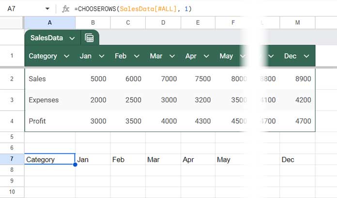
To get the last row from the same table, use the following formula:
=CHOOSEROWS(SalesData[#ALL], -1)The difference is minimal. The row_num argument in the first formula is 1, whereas in the second formula, it is -1.
Get the First or Last Column in a Table
Once you’ve tried extracting the first or last row in the new Google Sheets table, you can easily extract the first or last column.
What you want to do is replace CHOOSEROWS with CHOOSECOLS.
Syntax: CHOOSECOLS(array, [col_num1, …])
The following formula will help you get the first column in the table named “Purchase”:
=CHOOSECOLS(Purchase[#ALL], 1)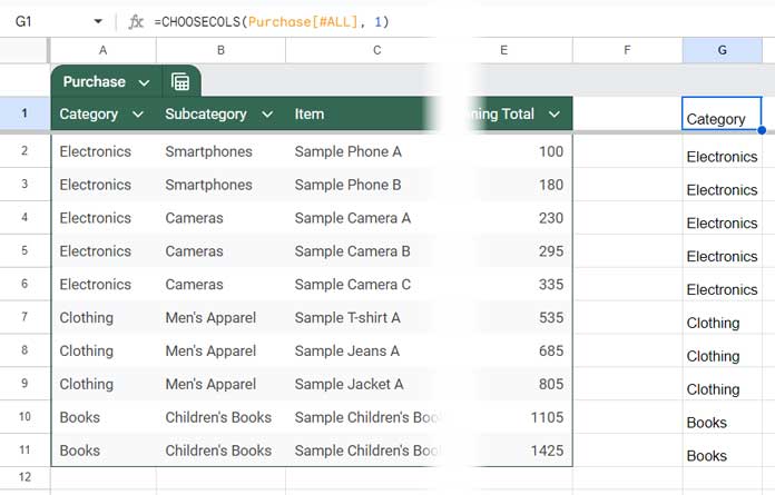
And the following one will help you find the last column in the same table:
=CHOOSECOLS(SalesData[#ALL], -1)Additional Tips: Finding the First or Last Cell Address of the New Google Sheets Table
We’ve utilized structured table references in all the above formulas, one of the beauties of the new table feature in Google Sheets.
How can you find the first or last cell address using the table name (structured table references)?
For example, let’s consider the above table named “Purchase”.
The following formula will return the cell address of the very first cell in the “Purchase” table:
=CELL("address", Purchase[#ALL]) // will return $A$1I’ve utilized the CELL function to return the ID, and the syntax is CELL(info_type, reference).
Where:
info_type: “address”reference: Purchase[#ALL]
To get the last cell address of the “Purchase” table, we will adopt a different approach that involves the ADDRESS function:
=ADDRESS(ROWS(Purchase[#ALL]), COLUMNS(Purchase[#ALL])) // will return $E$11This formula adheres to the syntax ADDRESS(row, column, [absolute_relative_mode], [use_a1_notation], [sheet]).
Where:
row: ROWS(Purchase[#ALL]) – it returns the number of rows in the tablecolumn: COLUMNS(Purchase[#ALL]) – it returns the number of columns in the table.
Resources
Here are some table-related resources in Google Sheets.