You can use several lookup functions to get the first text value in a range in Google Sheets. Additionally, you can find the first text value and retrieve the corresponding value from another range.

Here’s the simplest way to achieve this in Google Sheets:

=SINGLE(FILTER(range, ISTEXT(range)))

Replace range with the range from which you want to extract the first text value. This can be either a row or a column reference.

If you want to find the first text value in one range and get the corresponding value from another range, replace the filter range with the result range, and the second range (within ISTEXT) with the lookup range.

There are alternative solutions as well. We will explore those after an example.

Example of Getting the First Text Value

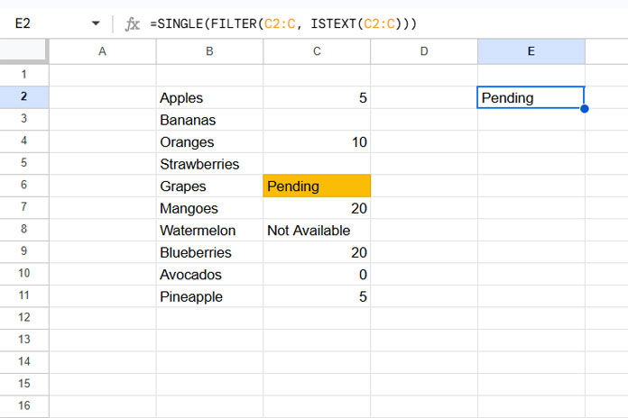
Consider the sample data where column B contains fruit names and column C contains available quantities. Some cells in C contain text, such as “Pending.”

The following formula will extract the first text value in C2:C:

=SINGLE(FILTER(C2:C, ISTEXT(C2:C)))

As per the sample data, this will return “Pending” in cell C6.

Here’s how the formula works:

• The ISTEXT function returns an array of TRUE or FALSE values, where TRUE represents text and FALSE represents other values.
• The FILTER function extracts all values corresponding to TRUE. In short, the FILTER function returns all text values.
• The SINGLE function (currently undocumented) returns only the first value from the filtered array.

Note: SINGLE is equivalent to using the + sign in front of the formula, like this: =+FILTER(C2:C, ISTEXT(C2:C)).

If you want to get the value from column B corresponding to the first text in column C, replace the filter range C2:C with B2:B. Here’s that formula:

=SINGLE(FILTER(B2:B, ISTEXT(C2:C)))

This will return “Grapes” from cell B6.

The formula works equally well for rows or columns. Simply adjust the references as needed.

Alternative Lookup Solutions

Here are two other great options for extracting the first text value in a range:

1. INDEX-XMATCH with ISTEXT

In this formula, we’ll use the ISTEXT function to return an array of TRUE/FALSE values:

=INDEX(C2:C, XMATCH(TRUE, ISTEXT(C2:C)))

• The XMATCH function finds the position of the first TRUE in the array returned by ISTEXT and returns its position.
• The INDEX function then uses that position to extract the value from C2:C.

Syntax: INDEX(reference, [row], [column])

In this formula, the reference is C2:C and the row is determined by the XMATCH function, i.e., XMATCH(TRUE, ISTEXT(C2:C)).

If you want to find the first text value in C2:C and return the corresponding value from B2:B, replace the reference C2:C with B2:B.

If you’re wondering whether you need to specify the XMATCH function in the column argument (when working with rows), the answer is no. When referring to a single row or column, the function automatically adapts to either a row (if the range is vertical) or a column (if horizontal).

2. XLOOKUP and ISTEXT Combo

Here’s another formula to get the first text value from a range:

=ARRAYFORMULA(XLOOKUP(TRUE, ISTEXT(C2:C), C2:C))

In this case, the role of ISTEXT is the same as before: it returns an array of TRUE/FALSE values corresponding to text and non-text values.

The XLOOKUP function uses this array as the lookup range. The search key is TRUE, and the result range is C2:C. The formula returns the first matching value from C2:C.

Syntax: XLOOKUP(search_key, lookup_range, result_range)

If you want the corresponding value in column B, replace C2:C (the result range) with B2:B.

Resources

• Get the First Numeric Value in a Range in Google Sheets
• Google Sheets: How to Return the First Non-blank Value in a Row or Column
• How to Lookup First and Last Values in a Row in Google Sheets
• Get the First and Last Row Numbers of Items in Google Sheets
• Get the Headers of the First Non-blank Cell in Each Row in Google Sheets
• XMATCH First or Last Non-Blank Cell in Google Sheets
• Excel: XLOOKUP for First and Last Non-Blank Value in Row