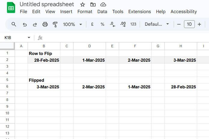
You can use the following formula to flip a row in Google Sheets while retaining empty cells:

=CHOOSECOLS(row, SEQUENCE(COLUMNS(row), 1, COLUMNS(row), -1))

Replace row with the row reference you want to flip. If you want to remove empty cells, you can use the FILTER function to exclude blanks.

Let’s first see how to flip a row in Google Sheets, then proceed to filtering out blank cells.

Example of Flipping a Row in Google Sheets

Assume you have the following values in A1:E1:

You can apply this formula in A2 to flip this row:

=CHOOSECOLS(A1:E1, SEQUENCE(COLUMNS(A1:E1), 1, COLUMNS(A1:E1), -1))

Output:

How Does This Formula Work?

Normally, the CHOOSECOLS function is used to extract specific columns from a range. For example:

=CHOOSECOLS(A1:E1, 5)

This returns the fifth column value in the range A1:E1.

If you specify a sequence of numbers from 5 to 1 in descending order:

=CHOOSECOLS(A1:E1, {5, 4, 3, 2, 1})

It effectively flips the row.

In the formula, I’ve used the SEQUENCE function to generate these numbers dynamically:

SEQUENCE(COLUMNS(A1:E1), 1, COLUMNS(A1:E1), -1)

Breakdown of SEQUENCE:

• COLUMNS(A1:E1) – Gets the total number of columns in the row.
• 1 – Number of columns in the sequence.
• COLUMNS(A1:E1) – The starting number (highest column index).
• -1 – Step value ensures the sequence decreases.

How to Remove Empty Cells While Flipping a Row

When working with growing datasets, you might prefer using dynamic row references like A1:1 or 1:1 instead of fixed ranges (A1:E1). However, this can introduce empty columns before the flipped row.

You can handle this in two ways:

1. Filtering out all empty cells (removes blanks anywhere in the row).
2. Trimming only trailing empty columns (keeps internal blanks intact).

Option 1: Remove All Empty Cells

=LET(
   ftr, CHOOSECOLS(A1:E1, SEQUENCE(COLUMNS(A1:E1), 1, COLUMNS(A1:E1), -1)), 
   FILTER(ftr, ftr<>"")
)

How It Works:

• The LET function stores the flipped row as ftr.
• FILTER(ftr, ftr<>"") removes all empty cells.

Result:

If there were empty cells in between, this method shifts data left to fill gaps.

Option 2: Remove Only Trailing Empty Cells

=ArrayFormula(CHOOSECOLS(A1:E1, SEQUENCE(XMATCH(TRUE, A1:E1<>"", 0, -1), 1, XMATCH(TRUE, A1:E1<>"", 0, -1), -1)))

How It Works:

• Instead of COLUMNS(A1:E1), we use: XMATCH(TRUE, A1:E1<>"", 0, -1)
  This finds the last non-empty column in the row.
• The sequence now starts from this position, ignoring trailing blanks.
• ARRAYFORMULA is applied since A1:E1<>"" is an array-based condition.

Key Difference from Option 1:

• Keeps empty cells in the middle of the row.
• Only removes trailing blanks.

Related Tutorials

• How to Flip a Column in Google Sheets – Finite and Infinite Columns
• How to Reverse an Array in Google Sheets [Fixed and Dynamic Array]
• FLIP in Google Sheets – Custom Named Function to Reverse Data
• Flip a Table Vertically in Excel (Includes Dynamic Array Formula)