")


")


")

")
")
 in Excel & Google Sheets")


If you need to implement dynamic product pricing in Google Sheets based on quantity, there are a few smart formula combinations that can help you automate the process. My go-to method is combining VLOOKUP with MATCH or XMATCH, but I’ll also walk you through a version using MAP and LAMBDA, just to show another way this can be done.
Let’s say you run a small office supplies store and want to offer different prices depending on how many units a customer orders. Instead of manually checking your tiered pricing chart, why not build a simple, automated solution in Google Sheets?
Sample Scenario
Suppose you sell products like pencils, pens, books, and color pencils. The price per item varies depending on the order quantity. For example:
- A Pen normally costs $2.00,
- But if someone orders 10 or more, the price drops to $1.25.
That’s quantity-based pricing, also known as tiered pricing, and it’s a great use case for automation in Google Sheets.
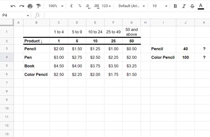
Here’s a sample price table (in range B2:G6):
| Product | 1 | 5 | 10 | 25 | 50+ |
|---|---|---|---|---|---|
| Pencil | $2.00 | $1.50 | $1.25 | $1.00 | $0.50 |
| Pen | $3.00 | $2.75 | $2.50 | $2.25 | $2.00 |
| Book | $5.00 | $4.00 | $3.75 | $3.50 | $3.25 |
| Color Pencil | $2.50 | $2.25 | $2.00 | $1.75 | $1.50 |
Now imagine your customer order list looks like this (in I3:J4):
| Product | Quantity |
|---|---|
| Pencil | 40 |
| Color Pencil | 100 |
Your goal is to return the correct unit price for each product based on quantity, in column K.
Try It Yourself: Open Sample Google Sheet
(Make a copy to test the formulas on your own)
Product Price Based on Quantity Using VLOOKUP and MATCH
Option 1: VLOOKUP with MATCH
This is the simplest and most recommended approach for handling dynamic pricing in Google Sheets.
Formula
=ArrayFormula(IFNA(VLOOKUP(I3:I4, B2:G6, MATCH(J3:J4, B2:G2, 1), 0)))This formula looks up the product name, finds the correct quantity tier using MATCH, and returns the corresponding price.
XMATCH Version
=ArrayFormula(IFNA(VLOOKUP(I3:I4, B2:G6, XMATCH(J3:J4, B2:G2, -1), 0)))XMATCH works similarly to MATCH, but offers a more intuitive syntax and better handling of approximate matches.
Tip: Make sure to clear cells
K3:K4before entering this formula to let the results spill automatically.
Product Price Based on Quantity Using INDEX, MATCH, and MAP
Option 2: Using INDEX and MATCH
This method is slightly more advanced but useful if you prefer using INDEX over VLOOKUP. It also shows how to apply a formula to multiple rows using MAP and LAMBDA.
Formula
=MAP(I3:I4, J3:J4, LAMBDA(a, b, IFNA(INDEX(B2:G6, MATCH(a, B2:B6, 0), MATCH(b, B2:G2, 1)))))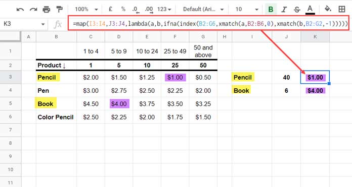
With XMATCH
=MAP(I3:I4, J3:J4, LAMBDA(a, b, IFNA(INDEX(B2:G6, XMATCH(a, B2:B6, 0), XMATCH(b, B2:G2, -1)))))This version loops through each product and quantity in the order list and returns the matching price based on the tiered pricing structure.
Behind the Formula
Let’s break down what’s actually happening when we calculate the price for, say, 40 Pencils.
How VLOOKUP Works
=VLOOKUP("Pencil", B2:G6, MATCH(40, B2:G2, 1), 0)Here’s how it works:
VLOOKUP("Pencil", B2:G6, …, 0)searches for “Pencil” in the first column of the price table.MATCH(40, B2:G2, 1)looks for the value 40 in the first row (which contains the quantity breakpoints: 1, 5, 10, 25, 50).- Since
MATCHis set to1(approximate match), it finds the largest value less than or equal to 40. - 40 falls between 25 and 50, so
MATCHreturns the 4th column, which corresponds to 25.
- Since
- So the formula simplifies to:
=VLOOKUP("Pencil", B2:G6, 4, 0)
…and returns $1.00, which is the correct unit price for 40 pencils.
In the array version, we wrap it in ARRAYFORMULA to apply this logic to all items in the order list.
How INDEX Works
=INDEX(B2:G6, MATCH("Pencil", B2:B6, 0), MATCH(40, B2:G2, 1))This works similarly:
MATCH("Pencil", B2:B6, 0)finds the row number for Pencil.MATCH(40, B2:G2, 1)finds the appropriate column based on the quantity.INDEXthen returns the value at that row and column intersection.
We use MAP and LAMBDA to apply this formula across the entire list.
Which Formula Should You Use?
- Stick with the VLOOKUP + MATCH combo if you’re looking for something clean, simple, and reliable.
- Go with the INDEX + MAP + LAMBDA method if you’re working with more complex dynamic pricing logic or just want to explore new functions.
Wrapping Up
That’s how you can set up dynamic product pricing in Google Sheets based on quantity. Whether you’re managing bulk pricing, tiered discounts, or just want to reduce manual work, these formulas can help automate your workflow with ease.
Give them a try—and feel free to tweak them to suit your setup.