To find the number of working and non-working days in a month or between two specific dates, you can use the NETWORKDAYS or NETWORKDAYS.INTL functions in Google Sheets.

If Saturday and Sunday are your weekends, you can use the NETWORKDAYS function. If you want to specify different weekends, use NETWORKDAYS.INTL. In the examples, I’ll use the NETWORKDAYS function.

If you’re not familiar with these functions, check out my related tutorial here: Google Sheets: The Complete Guide to All Date Functions.

Find the Total Number of Working Days in Google Sheets

Let’s look at the NETWORKDAYS function syntax:

NETWORKDAYS(start_date, end_date, [holidays])

The start_date and end_date arguments are mandatory to find the total network days in that period. To find the total number of working days in a specific month, simply provide the start date and calculate the end date using another function.

For example, let’s calculate the number of working days in the current month:

=NETWORKDAYS(EOMONTH(TODAY(), -1) + 1, EOMONTH(TODAY(), 0))

Enter this formula in a cell in your Google Sheets file, and it will return the total number of working days in the current month.

To find the total working days of any month, replace the TODAY() function with a specific date.

For example, if you want to find the total working days in November 2024, use any date from that month. Here’s the formula:

=NETWORKDAYS(EOMONTH("2024-11-28", -1) + 1, EOMONTH("2024-11-28", 0))

Formula Logic:

The key here is the EOMONTH function. From a provided date, we can find the end of the month date with this function. We can then use this as the end_date in the NETWORKDAYS formula.

The same function can be used to find the starting date of any month from a given date. For example:

=EOMONTH("2024-11-28", -1)

This formula returns the end date of the previous month. Adding one day to this result gives you the starting date of the current month or the month of the provided date. You can then use this as the start_date in the NETWORKDAYS function.

Note: You can enter holidays (dates other than weekends) in a separate column and reference that range in the formula to exclude those dates from the working day count. I’ll explain this in the later part of the tutorial.

Find the Total Number of Non-Working Days in Google Sheets

Once you’ve calculated the total number of working days, you can subtract this from the total days in the month to find the number of non-working days. If the last day of the month is the 30th, then the total number of days in that month is 30.

Here’s the formula to calculate the non-working days:

=DAY(EOMONTH(TODAY(), 0)) - NETWORKDAYS(EOMONTH(TODAY(), -1) + 1, EOMONTH(TODAY(), 0))

Let’s break down the first part of the formula:

=DAY(EOMONTH(TODAY(), 0))

This part of the formula returns the total number of days in the current month. To find the number of non-working days, you subtract the total working days (calculated using NETWORKDAYS) from this total.

Just like in the previous formula, you can replace TODAY() with any custom date to calculate non-working days for a specific month.

Conclusion

This is how you can find the number of working and non-working days in Google Sheets. Simply use the NETWORKDAYS function to calculate the working days and subtract that from the total days in the period to find the non-working days.

In the following example, the start date is in cell B2, the end date is in cell B3, and the holidays are listed in range B5:B9.

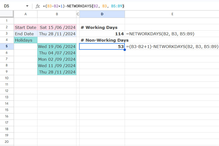
The following formula returns the number of working days during this period:

=NETWORKDAYS(B2, B3, B5:B9)

And this formula returns the number of non-working days in the period:

=(B3-B2+1)-NETWORKDAYS(B2, B3, B5:B9)

Here, (B3-B2+1) calculates the number of days between the start date and end date, both inclusive.

Resources

• Return All Working Dates Between Two Dates in Google Sheets
• How to Highlight Next N Working Days in Google Sheets
• Finding the Last 7 Working Days in Google Sheets (Array Formula)
• Last Working Day of a Given Year – Google Sheets Formula
• Get Last Saturday of Any Given Month and Year in Google Sheets
• How to Find the Last Business Day of a Month in Excel
• Same Day Last Week Comparison in Google Sheets