We can use a criteria list for filtering a table based on multiple conditions in Google Sheets. But what if this list contains wildcards (? and *)?
To handle such scenarios, we can employ the QUERY function in Google Sheets to filter data based on the criteria list with wildcards.
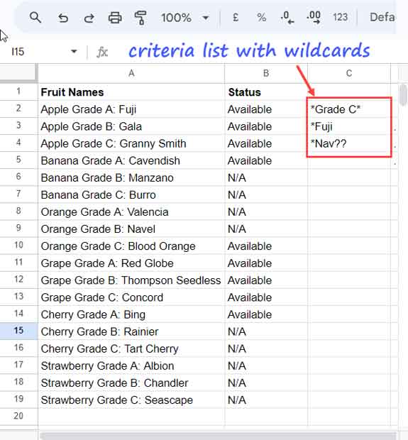
For this example, let’s consider a table containing fruit names with grades in column A and their availability in column B.
The data range is precisely A1:B19, where A1:B1 contains the field labels ‘Fruit Names’ and ‘Status,’ respectively. The criteria list with wildcards is in C2:C4, comprising *Grade C*, *Fuji, and *Nav??, respectively.

Our goal is to filter the rows based on this criteria list that contains wildcard characters in Google Sheets.
Specifically, we aim to filter items (fruit names) that do not contain Grade C, do not end with Fuji, and do not end with Nav followed by any two characters.
Filter Rows Based on Criteria List with Wildcards: Step-by-Step Instructions
Here are three steps involved in this process:
- Substituting Wildcard Characters
For this type of filtering in Google Sheets, we will use the MATCHES (preg) regular expression match in the QUERY function.
To begin, we need to substitute the wildcard character asterisk (*) with (.*), and the question mark (?) with (.).
.: Matches any single character except for a new line.*: Matches 0 or more occurrences of the preceding character (in this case, the dot).
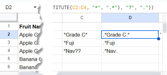
Our criteria list with wildcards is in C2:C4. In D2, insert the following nested SUBSTITUTE formula to make these changes.
=ArrayFormula(SUBSTITUTE(SUBSTITUTE(TOCOL(C2:C4, 1), "*", ".*"), "?", "."))The TOCOL function here is used to eliminate any empty cells in the criteria range.
Please see the output of this substitution in the screenshot below.

- Creating a Regular Expression Pattern
To perform multiple criteria filtering in Google Sheets with filter criteria in a range and also containing wildcards, we have replaced the wildcards with supporting regular expression wildcards.
Now, combine those criteria separated (delimited) by a pipe.
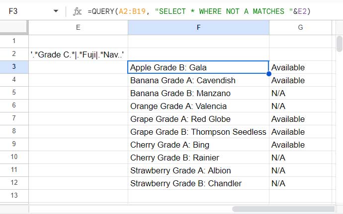
="'"&TEXTJOIN("|", TRUE, D2:D4)&"'"This TEXTJOIN function in cell E2 joins the criteria with wildcards in D2:D4 and places a pipe delimiter in between. If any cell in this range is blank, the function will omit that cell.
Output:'.*Grade C.*|.*Fuji|.*Nav..'
- Filter Rows Based on the Criteria List with Wildcards
The following QUERY formula filters rows where column A in the range doesn’t match the criteria.
=QUERY(A2:B19, "SELECT * WHERE NOT A MATCHES "&E2)
If you want to filter rows matching the criteria, use the one below.
=QUERY(A2:B19, "SELECT * WHERE A MATCHES "&E2)The first formula uses the NOT logical operator, whereas the second one doesn’t.
How to Escape Wildcards in the Data Range to Filter
Sometimes, your rows to filter (records in the table) may contain wildcard characters that you need to treat literally, such as a question mark at the end of a string.
Usually, we use the tilde in such cases. For example, to match Available? we will use Available~?.
However, in a MATCHES regular expression match, the tilde won’t work. Instead, you should use the backslash.
So, when you filter rows based on a criteria list with wildcards, do not include such criteria in the list (here in C2:C4). Instead, place them below the list in D2:D4. This is because we don’t want to perform the substitution of wildcards with MATCHES supported wildcards.
For example, if you want to match any text that ends with Apple?, enter .*Apple? in D5. Accordingly, the range in the formula in E2 should be modified from D2:D4 to D2:D5.
Resources
Above, we utilized the MATCHES function in QUERY to filter rows in a table based on a criteria list with wildcards in Google Sheets. Here are guides on performing complex string comparison operators in Google Sheets, aside from using MATCHES.


