


")


")

")
")
 in Excel & Google Sheets")


Have you ever needed to find numbers where each digit appears only once? That’s exactly what this tutorial is about — how to filter (also highlight) unique digit numbers in Google Sheets.
Think of numbers like 12345 — every digit is different. But 12344? That one repeats the digit 4, so it doesn’t qualify. This trick is surprisingly useful in real life! I’ve used it to check serial numbers, spot cleaner data entries, and even for fun stuff like analyzing lottery picks.
Whether you’re working with PINs, raffle entries, product IDs, or just enjoy playing with numbers, this method helps you quickly identify the ones that stand out — without any repeats.
In this post, I’ll walk you through how to filter (also highlight) unique digit numbers in Google Sheets using formulas, step by step.
Let’s dive in!
How to Filter Unique Digit Numbers in Google Sheets
Assume you have PINs in column B (starting from B2) and you want to filter all the unique digit PINs from this list.
Example Data:
| PIN Numbers |
| 1234 |
| 4456 |
| 3216 |
| 6548 |
| 4425 |
You can use the following formula to filter numbers with all unique digits:
=FILTER(B2:B, MAP(B2:B, LAMBDA(row, LEN(row)=COUNTA(UNIQUE(MID(row, SEQUENCE(LEN(row)), 1))))))Output:
| Unique PINs |
| 1234 |
| 3216 |
| 6548 |
If you're using this formula for a different range, replace B2:B with your actual range.
Formula Explanation
Let’s break it down:
MID(row, SEQUENCE(LEN(row)), 1)– splits each digit of the number into separate cells.UNIQUE(...)– removes any repeated digits.COUNTA(...)– counts how many unique digits remain.LEN(row)=COUNTA(...)– returnsTRUEonly if all digits were unique (i.e., length of the number equals count of unique digits).MAP(...)– applies this logic to every row in the given range.FILTER(...)– returns only the rows for which the above logic isTRUE.
That’s how the formula filters unique digit numbers in Google Sheets.
How to Highlight Unique Digit Numbers in Google Sheets
To highlight unique digit numbers in the range B2:B:
- Select the range
B2:B. - Go to Format > Conditional formatting.
- Under “Format rules,” choose Custom formula is.
- Enter this formula:
=LEN(B2)=ARRAYFORMULA(COUNTA(UNIQUE(MID(B2, SEQUENCE(LEN(B2)), 1)))) - Set your formatting style.
- Click Done.
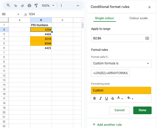
Now, all numbers with unique digits in the selected range will be highlighted!
Resources – Other Interesting Google Sheets Tips
- How to Split a Number into Digits in Google Sheets
- Allow Only N Digits in Data Validation in Google Sheets (Accept Leading Zeros)
- How to Generate a List of Strong Passwords in Google Sheets
- Formula to Generate Unique Readable IDs in Google Sheets
- How to Generate Barcodes in Google Sheets (Code 39)
- Create Your Own Ciphers in Google Sheets