Creating unique IDs in Google Sheets doesn’t always have to mean lifeless numbers or random characters. Instead, you can generate Unique Readable IDs in Google Sheets using formulas — no Apps Script needed.

These IDs can be purely numeric or alphanumeric and structured in a way that’s meaningful and easy to interpret, like embedding parts of a product’s category, vendor, or even its position in a list. Let me show you how.

Examples of Creating Unique Readable IDs in Google Sheets

Let’s walk through a couple of examples. You can tweak the formulas to fit your actual use case — I’ll explain how at the end.

Example 1: Unique Readable IDs for Books Bought

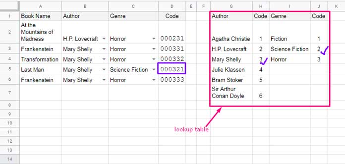
Suppose you’re maintaining a list of books with their authors and genres. Here’s one such record:

• Book: Last Man
• Author: Mary Shelly
• Genre: Fiction

In this setup, each unique readable ID we generate will consist of:

• A code for the author
• A code for the genre
• A running count for that author + genre combo

Say, for the book above, the resulting ID is 000321 (cell D5). Here’s what it means:

• 3 → Author code (from a lookup table)
• 2 → Genre code (from a lookup table)
• 1 → This is the first book under that author + genre

And those leading zeros? They’re just formatting — they don’t carry any meaning but help keep your IDs uniform.

Sample Lookup Tables

In the same sheet (or another sheet), create lookup tables like this:

You can expand these as needed. The formula will adjust automatically.

ID Formula (Step-by-Step)

Let’s break it down. You’ll need three formulas that we’ll eventually combine:

1. Lookup Author Codes

=ArrayFormula(XLOOKUP(B2:B, G2:G, H2:H))

This looks up the Author in column B against the lookup table in column G and returns the corresponding code from column H.

2. Lookup Genre Codes

=ArrayFormula(XLOOKUP(C2:C, I2:I, J2:J))

Same idea — match Genre and pull the genre code.

3. Count Occurrences of Each Author + Genre Combo

=ArrayFormula(COUNTIFS(B2:B&C2:C, B2:B&C2:C, ROW(A2:A), "<="&ROW(A2:A)))

This counts how many times a given Author + Genre combo appears up to each row.

4. Combine and Format

Bring it all together:

=ArrayFormula(
   IF(A2:A="", , 
      TEXT(
         XLOOKUP(B2:B, G2:G, H2:H) & 
         XLOOKUP(C2:C, I2:I, J2:J) & 
         COUNTIFS(B2:B&C2:C, B2:B&C2:C, ROW(A2:A), "<="&ROW(A2:A)), "000000"
      )
   )
)

This formula:

• Ignores blank rows
• Returns a 6-digit unique readable ID for each record

Paste it in D2, and you’re good to go.

Example 2: Unique Readable IDs for Assets Purchased

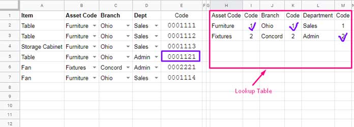
Now let’s scale things up. Suppose you want to include three fields in your ID — say:

• Item Type (e.g., Furniture)
• Branch (e.g., Ohio)
• Department (e.g., Admin)

We can apply the same logic, just with one more lookup and a slightly longer format.

Sample Output

Let’s say for a table purchased for the Admin department at the branch office in Ohio, the ID is 0001121:

• 1 → Item Type code
• 1 → Branch Code
• 2 → Department code
• 1 → First occurrence of this combination

3-Lookup ID Formula

Here’s the full formula:

=ArrayFormula(
   IF(A2:A="", , 
      TEXT(
         XLOOKUP(B2:B, H2:H, I2:I) & 
         XLOOKUP(C2:C, J2:J, K2:K) & 
         XLOOKUP(D2:D, L2:L, M2:M) & 
         COUNTIFS(B2:B&C2:C&D2:D, B2:B&C2:C&D2:D, ROW(A2:A), "<="&ROW(A2:A)), "0000000"
      )
   )
)

What’s happening here:

• We’re looking up three values: Item Type (B), Branch (C), Department (D)
• Then counting how many times that trio has appeared so far
• And formatting the result to be a 7-digit ID

Bonus: How to Create Alpha-Numeric Readable IDs in Google Sheets

Want readable IDs with letters in them? You can — just use alphabets in your lookup tables instead of numbers.

For example:

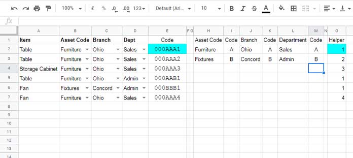
Now the generated ID could be something like 000AAB1 — representing a piece of furniture for the Admin department at the Ohio branch, and it’s the first entry of that combination.

However, since TEXT won’t work as expected on alphanumeric codes, pad the zeros manually:

=ArrayFormula(
   IF(A2:A="", , 
      "000" & 
      XLOOKUP(B2:B, H2:H, I2:I) & 
      XLOOKUP(C2:C, J2:J, K2:K) & 
      XLOOKUP(D2:D, L2:L, M2:M) & 
      COUNTIFS(B2:B&C2:C&D2:D, B2:B&C2:C&D2:D, ROW(A2:A), "<="&ROW(A2:A))
   )
)

You can adapt either of these examples for your inventory, asset tracking, library, or product management needs — wherever you want to auto-generate unique readable IDs in Google Sheets.

Resources

• How to Generate Barcodes in Google Sheets (Code 39)
• How to Generate a List of Strong Passwords in Google Sheets
• Create Your Own Ciphers in Google Sheets