


")


")

")
")
 in Excel & Google Sheets")


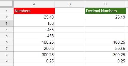
Imagine you have a list in Google Sheets containing a mix of decimal and integer numbers. How can you filter only the decimal numbers from this list?
This is Question #1, which I’ll answer in this tutorial. As a bonus, I’ll also tackle Question #2:
How can you filter decimal numbers with specific decimal fractions?
For example, filtering numbers with a fraction of 0.25—but you can easily modify this to suit your needs.
Formula to Filter Decimal Numbers in Google Sheets
To filter decimal numbers, we’ll use the INT function along with either IF or FILTER. Both approaches achieve the same goal but produce slightly different outputs:
- INT with IF: May leave blank cells in the results where no match is found.
- INT with FILTER: Returns only the matching values without blank cells.
First, let’s learn how to filter decimal numbers. Then, we’ll cover how to filter numbers with specific decimal fractions. The formulas for both are nearly identical, with the main difference being the comparison operator used.
How to Filter Decimal Numbers in Google Sheets
Here’s the formula to extract decimal numbers:
=ArrayFormula(IF(A2:A-INT(A2:A)<>0, A2:A, ))- The range
A2:Acontains the input data. - Use this formula in cell
B2. - Before applying the formula, ensure the range
B2:Bis clear of any values or formulas.
Alternatively, you can use the FILTER function to achieve the same result:
=FILTER(A2:A, A2:A-INT(A2:A)<>0)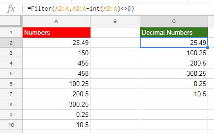
Both formulas will do the job, but the FILTER version excludes blank rows.
Additional Tip
If you apply the above formulas to a column containing dates and timestamps, they will return the timestamps. This is because dates in Google Sheets are stored as integers, while times are stored as fractions of a day. Therefore, a timestamp is treated as a decimal number.
Filter Specific Decimal Fractions in Google Sheets
To filter decimal numbers with a specific fraction (e.g., 0.25), modify the formula as follows:
Formula #1 (Using INT with IF):
=ArrayFormula(IF(A2:A-INT(A2:A)=0.25, A2:A, ))Formula #2 (Using INT with FILTER):
=FILTER(A2:A, A2:A-INT(A2:A)=0.25)Both formulas will return numbers with the desired fraction (e.g., 0.25). For instance, if the dataset contains 100.25, 300.25, and 0.25, these numbers will appear as output.
Key Takeaways
To filter decimal numbers in Google Sheets, you can combine the INT function with either IF or FILTER. This approach effectively separates decimal numbers from integers in your data.
If you need to filter specific decimal fractions, you can adjust the formula by replacing 0.25 with your desired fraction. This allows for precise filtering tailored to your requirements.
For cleaner outputs without blank cells, the FILTER function is the ideal choice, as it directly excludes non-matching values.