How to Filter Current Week Horizontally in Google Sheets

Published on

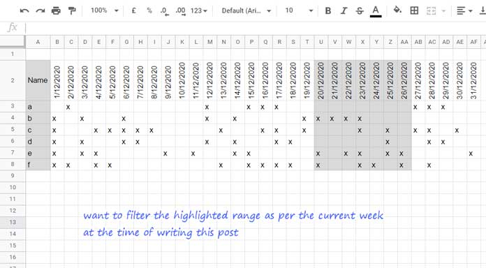
First of all, you must know what I meant by filter the current week horizontally in Google Sheets.

Assume you have a dataset that contains several columns and the column headers are dates. That means the first row in your dataset will be the header row with dates.

You want to filter only the columns in which the header row contains dates that fall in the current week. That’s what I meant by filter the current week horizontally in Google Sheets.

Suitable Functions

For our purpose, we can use two functions that have the filtering ability. They are none other than the Query and Filter.

Other than these, to find the week number of the current week, we may also require the Weeknum function.

Since the Weeknum function is not part of Query, we may require to follow a workaround for such types of filtering of data.

Must Check: How to Utilize Google Sheets Date Functions [Complete Guide].

But the FILTER function supports horizontal filtering and also the Weeknum function. So, we can directly use Weeknum based criteria within the Filter.

In this post, let’s learn how to filter dates that fall in the current week in the header row in Google Sheets. First I’ll use the FILTER, then we can go to the QUERY.

Sample Data:

Data Sample

Filter Function to Filter the Current Week Horizontally

There are two steps involved in this type of horizontal filtering in Google Sheets.

  1. Filter the columns that contain the dates that fall in the current week in the header row.
  2. Combine the text column (here, the first column) with the filtered result.

Let’s first filter the current week horizontally in Google Sheets using the below Filter formula.

=filter(B2:AF,weeknum(B2:AF2)=weeknum(today()))

Insert the above Filter formula in cell AH2 to filter the dataset horizontally based on the Weeknum criteria.

Syntax of the function FILTER (as per our formula above) for your quick reference:

FILTER(range, condition1)

range (the range to filter): B2:AF

condition: weeknum(B2:AF2)=weeknum(today())

Finally, combine the first text column with the filtered result. For that, edit the just above Filter formula as below.

={A2:A,filter(B2:AF,weeknum(B2:AF2)=weeknum(today()))}
Filter Current Week Horizontally in Google Sheets

This way, we can use the Filter function to filter the current week (current week’s data) horizontally in Google Sheets.

Query Current Week’s Data Horizontally

Usually, we use the Query function to filter vertically. I mean filter a column or multiple columns based on the values in those columns.

If the date column is the first column, we can easily use the Query to filter the rows based on the dates in that column. But there is no Weeknum scalar function in Query.

That means to Query (filter) current week horizontally or vertically, we need to depend on the Weeknum function.

Here I am going to use a workaround method to filter/query the current week horizontally. Here is how.

Logic

In the SELECT clause in the Query function, we can specify the columns to filter.

Eg.:

=query({A2:AF},"Select Col1, Col2")

First, see the above Filter formula result. Based on that, we need to filter Column 1 and columns 21 to 27.

Cell U2 (the 21st column) contains the start date of the current week, and cell AA2 (27th column) contains the end date of the current week.

To Query Current Week Horizontally, we must first find the above column numbers dynamically. Here are the steps to follow.

Note:- I suggest you use the FILTER method. This QUERY method is for educational purposes as it’s a little complex in nature.

Steps

Two Match Formulas to Find the Column Numbers

Match_Formula_1

1. Insert the below MATCH formula in cell AH1 to return the starting column number of the current week. The formula would return 21.

=ArrayFormula(match(weeknum(today()),weeknum(A2:AF2),0))

Match_Formula_2

2. Insert the below MATCH formula in cell AI1 to return the ending column number of the current week. The formula would return 27.

=ArrayFormula(match(weeknum(today()),weeknum(A2:AF2),1))

Both the Match formulas are the same except for the last argument.

Can you explain the formulas to us?

Yes! Here you go.

Syntax of the function MATCH for your quick reference:

MATCH(search_key, range, search_type)

The last argument in the formula, i.e., search_type, 0, treats the range as unsorted (even if it’s a sorted range). So it would return the exact match of the value (Weeknum) found in the starting of the range (the result is 21).

If it’s (search_type) 1, the formula treats the range as a sorted range and would return the largest value less than or equal to search_key (Weeknum). So the last match will be returned (the result is 27).

Note:- The first row in the dataset that contains the dates must be sorted in ascending order. Otherwise, the above Match formulas won’t work correctly.

Query Clause to Filter Current Week Horizontally

Now we need to write the formula as below to filter current week horizontally in Google Sheets.

=query({A2:AF},"Select Col1, Col21, Col22, Col23, Col24, Col25, Col26, Col27",1)

To make the formula part in bold letters dynamic, we can use the above match formulas as below.

Steps to Follow:

Let’s write a Sequence formula to replace Col21, Col22, Col23, Col24, Col25, Col26, Col27 in the above formula.

=sequence(AI1-AH1+1,1,AH1)

SEQUENCE syntax for your quick reference:

SEQUENCE(rows, columns, start)

rows (number of rows to return) – AI1-AH1+1 (it means match_formula_2-match_formula_1+1)

columns (number of columns to return) – 1

start (sequence starting from) – AH1 (match_formula_1)

To skip using the helper cells AH1 and AI1, we can rewrite the above formula as below.

=sequence(
     ArrayFormula(match(weeknum(today()),weeknum(A2:AF2),1))-
     ArrayFormula(match(weeknum(today()),weeknum(A2:AF2),0))+1,
     1,
     ArrayFormula(match(weeknum(today()),weeknum(A2:AF2),0))
)
Query to Filter Current Week Horizontally - Dynamic Select

We should modify the above formula further to make it as the Query clause text Col21, Col22, Col23, Col24, Col25, Col26, Col27.

Here is the modified formula.

=textjoin(
     ",",true,
     ArrayFormula(
        "Col"&sequence(
           ArrayFormula(match(weeknum(today()),weeknum(A2:AF2),1))-
           ArrayFormula(match(weeknum(today()),weeknum(A2:AF2),0))+1,
           1,
           ArrayFormula(match(weeknum(today()),weeknum(A2:AF2),0))
        )
     )
)

We just need only one ArrayFormula in the above formula. So we can shorten it as below and let’s call it dynamic_select_formula.

Dynamic_Select_Formula

=ArrayFormula(
     textjoin(
        ",",true,
        "Col"&sequence(
           match(weeknum(today()),weeknum(A2:AF2),1)-
           match(weeknum(today()),weeknum(A2:AF2),0)+1,
           1,
           match(weeknum(today()),weeknum(A2:AF2),0)
        )
     )
)

Here is the non-dynamic Query formula to filter the current week’s data horizontally in Google Sheets.

=query({A2:AF},"Select Col1, Col21, Col22, Col23, Col24, Col25, Col26, Col27",1)

Just delete the formula part Col21, Col22, Col23, Col24, Col25, Col26, Col27",1).

So the formula would look like as below.

=query({A2:AF},"Select Col1,

Change it as below.

=query({A2:AF},"Select Col1,"&

Then copy paste the above dynamic_select_formula at the end part of the above formula.

=query({A2:AF},"Select Col1,"&ArrayFormula(textjoin(",",true,"Col"&sequence(match(weeknum(today()),weeknum(A2:AF2),1)-match(weeknum(today()),weeknum(A2:AF2),0)+1,1,match(weeknum(today()),weeknum(A2:AF2),0)))))

That’s all. The above are the two methods to filter current week horizontally in Google Sheets.

Enjoy!

Prashanth KV
Prashanth KV
Your Trusted Google Sheets and Excel Guide Prashanth KV brings a wealth of experience in Google Sheets and Excel, cultivated through years of work with multinational corporations in Mumbai and Dubai. As a recognized Google Product Expert in Docs Editors, Prashanth shares his expertise through insightful blogging since 2012. Explore his blog for practical tips and guidance on maximizing your spreadsheet skills.

Highlight Upcoming Birthdays in Google Sheets

When highlighting upcoming birthdays in Google Sheets, one important aspect is ignoring the year...

Compare Two Tables for Differences in Excel

To compare two tables with similar data for differences, you can use the XLOOKUP...

Calculate Weighted Average in Pivot Table in Google Sheets

You can calculate a weighted average in a Pivot Table using a custom formula...

Summarize Data and Keep the Last Record in Google Sheets

In Google Sheets, we can summarize data (like sum, average, min, max, count) using...

More like this

Highlight Upcoming Birthdays in Google Sheets

When highlighting upcoming birthdays in Google Sheets, one important aspect is ignoring the year...

Calculate Weighted Average in Pivot Table in Google Sheets

You can calculate a weighted average in a Pivot Table using a custom formula...

Summarize Data and Keep the Last Record in Google Sheets

In Google Sheets, we can summarize data (like sum, average, min, max, count) using...

LEAVE A REPLY

Please enter your comment!
Please enter your name here

This site uses Akismet to reduce spam. Learn how your comment data is processed.