How to Extract Numbers But Ignore Dates in Google Sheets

In this tutorial, you’ll learn how to extract numbers from a mixed data range in Google Sheets while ignoring dates—even though dates are technically stored as numbers in Sheets.

That’s right—Google Sheets treats dates as serial numbers behind the scenes, which can make it tricky when you’re trying to filter just the plain numbers. Fortunately, we’ve got two solutions:

One that uses a LAMBDA helper function (ideal for smaller datasets)
Another without LAMBDA (better for larger ranges due to better performance)

Let’s look at an example and then go through both formulas.

Table of Contents

Sample Mixed Data for Extracting Numbers in Google Sheets

Mixed Data
123
2024-07-01
Invoice #456
789
01/15/2025
Apples
321
$100
2025-01-01
654

From this list, we want to extract just the numeric values like 123, 789, 321, 100, and 654, while excluding dates and text.

Extract Numbers But Ignore Dates Using LAMBDA

If you have a mix of data types in a column like A2:A, you can use the following formula in B2 to extract only the non-date numbers:

=MAP(A2:A, LAMBDA(cell, IF(AND(ISNUMBER(cell), NOT(ISDATE(cell))), cell,)))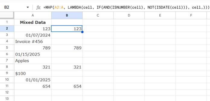

LAMBDA function extracting numbers, excluding dates

You can apply this to a 2D range like A2:B without changing the formula—just update the range reference:

=MAP(A2:B, LAMBDA(cell, IF(AND(ISNUMBER(cell), NOT(ISDATE(cell))), cell,)))

💡 New to LAMBDA in Google Sheets? Check out How to Use the LAMBDA Function in Google Sheets (Standalone) for a beginner-friendly guide.

Formula Breakdown

AND(ISNUMBER(cell), NOT(ISDATE(cell))) – This checks whether a cell contains a number and is not a date.
IF(..., cell,) – If the condition is true, return the value; otherwise, return blank.
MAP(...) – Applies the above logic to every cell in the range.

Note: We use MAP because ISDATE doesn’t evaluate arrays element-wise. It only returns TRUE if all values are dates, and FALSE otherwise. So, to individually test each cell, we need a LAMBDA with MAP.

Extract Numbers But Ignore Dates Without LAMBDA

Want a more efficient approach for large datasets? Use this ArrayFormula that doesn’t rely on MAP or LAMBDA:

=ArrayFormula(IF(ISNUMBER(A2:A)*NOT(IFERROR(DATEVALUE(A2:A))), A2:A, ))

Formula Breakdown

Let’s break it down step by step:

ISNUMBER(A2:A)
Returns TRUE for all cells that contain numeric values—including both plain numbers and dates (since dates are stored as serial numbers).
DATEVALUE(A2:A)
Tries to convert each cell to a date.
- Returns a numeric serial value for actual dates or valid date strings.
- Returns an error for anything that isn’t a valid date (e.g., plain numbers, text like “Apples”, or strings like “Invoice #456”).
IFERROR(DATEVALUE(A2:A))
Suppresses the errors from DATEVALUE.
- For non-date values, it now returns blank instead of an error.
- For valid dates, it still returns a number.
NOT(IFERROR(DATEVALUE(...)))
- Turns date values into FALSE.
- Turns everything else (non-date values like numbers or text) into TRUE.
ISNUMBER(...) * NOT(...)
- Multiplying the two booleans acts like a logical AND.
- Only cells that are numbers and not dates result in TRUE.
IF(..., A2:A, )
Returns the original value from column A only if the result is TRUE, otherwise returns blank.

This method excludes date values by checking if a number does not successfully convert to a date.

Optional: Remove Blank Cells from the Output

When you’re working with a one-dimensional range and want to eliminate blank results, wrap the formula in TOCOL:

LAMBDA version with TOCOL:

=TOCOL(MAP(A2:A, LAMBDA(cell, IF(AND(ISNUMBER(cell), NOT(ISDATE(cell))), cell,))), 3)

Non-LAMBDA version with TOCOL:

=ArrayFormula(TOCOL(IF(ISNUMBER(A2:A)*NOT(IFERROR(DATEVALUE(A2:A))), A2:A, ), 3))

TOCOL(..., 3) flattens the array vertically while skipping blanks.
This also works with 2D ranges, though the result will be flattened into a single column.

When to Use Which Formula?

Use Case	Recommended Formula
Small dataset, flexible range (1D or 2D)	`MAP + LAMBDA`
Large dataset, performance matters	`ArrayFormula + DATEVALUE`
Need a clean list with no blanks	Wrap with `TOCOL(...)`