Sometimes we may require to extract search keys and Vlookup in Google Sheets. In this Google Sheets tutorial, you can learn how to do this. Before that, I would like to darg your attention to a different scenario in the vertical lookup (Vlookup)!
What’s that?
If a ‘search key’ is part of a text (substring) in the lookup table (first column in the ‘range’), then we can use wildcard characters with the search key.
Vlookup Syntax for Reference: VLOOKUP(search_key, range, index, [is_sorted])
Though I’ve explained the same in my post titled Partial Match in Vlookup in Google Sheets, here is one example.
After this example, I’ll come to our topic of this post, i.e. how to extract search keys and Vlookup in a table in Google Sheets.
| First and Last Name | Advance |
| Martha Thompson | 5400 |
| Diana Reed | 5000 |
| Harold Scott | 0 |
Copy this table and paste it into cell A1 in your new sheet.
Assume you want to find the advance paid to “Diana Reed”. You have the search key “Diana”.
Here is the partial match Vlookup using a wildcard character. Do take note of the asterisk character usage with the search key.
=vlookup("*Diana*",A1:B4,2,0)In this Google Sheets tutorial, what we are going to do is the reverse of this.
I mean the search key is “Diana Reed” (first and last name or full name) but the lookup table column 1 has only the first names.
Here we must require to extract the search key and then do the Vlookup.
In Google Sheets, for this, we can use the Regexextract function with the Vlookup function here.
When Should One Extract Search Keys and Vlookup in Google Sheets?
I have already touched the scenario above. Now, here is one example (range A1:B4).
| First Name | Advance |
| Martha | 5400 |
| Diana | 5000 |
| Harold | 0 |
My search key for vertical lookup here is “Diana Reed”. If I use the below Vlookup formula, no doubt it would return #N/A.
=vlookup("Diana Reed",A1:B4,2,0)The reason, the search key is not available in the first column of the lookup table.
In concise, I have the first name and last name together as the search key to Vlookup a table that contains only the first names.
By extracting the search key, i.e. first name, we can do this type of vertical lookup.
Didn’t get?
Example
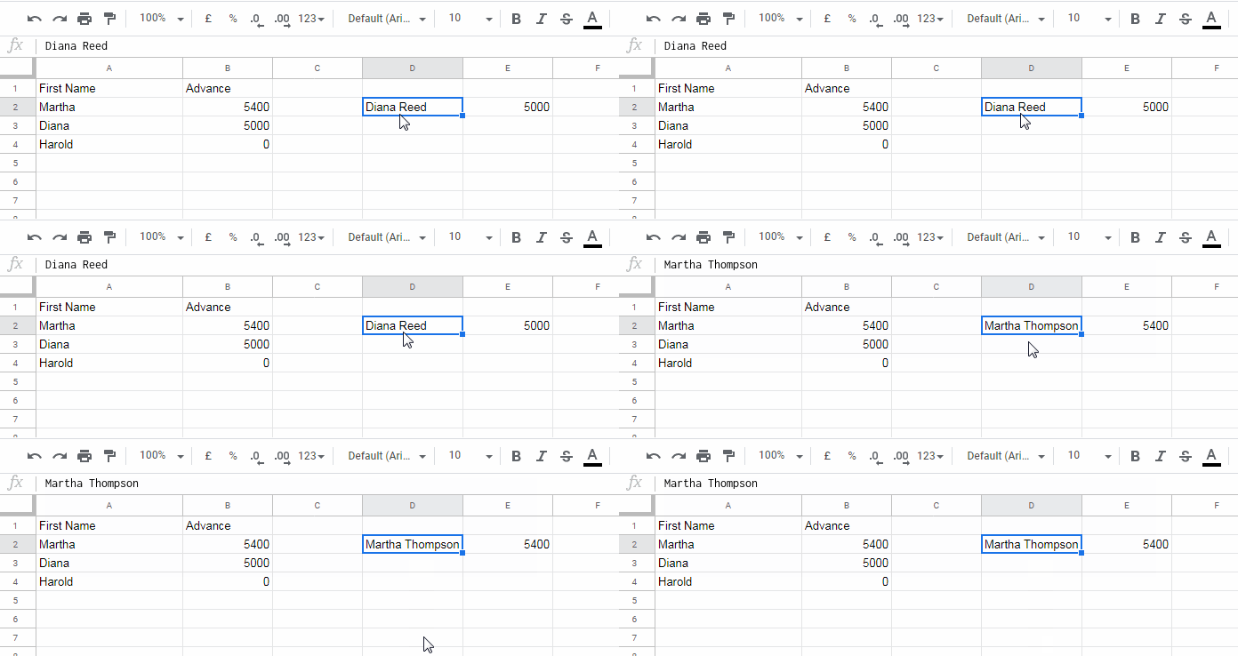
See the full name as the search key in cell D2. Let’s see how to systematically extract the search key (first name) only from this and use it in Vlookup in the cell E2.

When I say systematically extracting a search key, I mean to say match first names (A2:A4) in first and last name (D2) and extract matching string from D2.
How to extract search keys as above and Vlookup in a table in Google Sheets?
Extract Search Key for Vlookup in Google Sheets
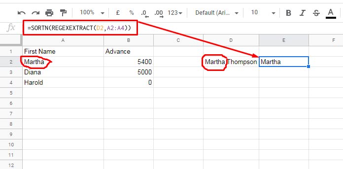
Use the below Regexextract + Sortn formula for extracting the search key as per the above explanation.
=SORTN(REGEXEXTRACT(D2,A2:A4))If “Martha Thompson” is the Vlookup search key, the formula would extract “Martha” after matching the first names in column A with the name in cell D2.

Let’s use this (the formula) as the search key in Vlookup.
FORMULA 1:
=vlookup(SORTN(REGEXEXTRACT(D2,A2:A4)),A1:B4,2,0)That’s all!
How Do We Extract Multiple Search Keys and Vlookup Them in Google Sheets?
Some times we may require to use multiple search keys in Vlookup in Google Sheets. I mean to return a Vlookup array result.
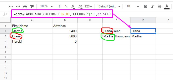
This time, in my example, I have two search keys to extract. They are the first and last names as below in D2 and D3.

We can extract multiple search keys for Vlookup using the below Regexextract + Textjoin formula. The earlier one (Regexextract + Sortn) won’t work here.
=ArrayFormula(REGEXEXTRACT(D2:D3,TEXTJOIN("|",1,A2:A4)))Let’s use the above formula as the search keys in Vlookup (the ArrayFormula moved).
FORMULA 2:
=ArrayFormula(vlookup(REGEXEXTRACT(D2:D3,TEXTJOIN("|",1,A2:A4)),A2:B4,2,0))The Vlookup formula above in cell E2 would return 5000 in cell E2 and 5400 in cell E3.
Conclusion
In real life, we can use the above Vlookup to assign values to a table. For example, I have a column (Sheet1!A1:A) with campaign names as follows.
A1: Conversion – Remarketing Dynamique.
A2: Conversion – Loyalty marketing.
A3: Conversion – Loyalty marketing.
A4: Conversion – Remarketing Dynamique.
In the same sheet B1:B (Sheet1!B1:B), I want to assign campaign types from a table that looks likes below (Sheet2!A1:B).
| Campaign Name | Campaign Type |
| Remarketing | Type 1 |
| Loyalty marketing | Type 2 |
Here we can use the below formula that’s in line with our FORMULA 2 above.
=ArrayFormula(IFNA(vlookup(REGEXEXTRACT(A1:A,TEXTJOIN("|",1,Sheet2!A2:A4)),Sheet2!A2:B4,2,0)))Note: Used IFNA function additionally as both the ranges are open. An open range may cause #N/A errors. The said function makes such errors blank.
That’s all about how to extract search keys and Vlookup in Google Sheets. Thanks for the stay, enjoy!


Hi Prashanth! I have learned so much from so many of your tutorials! Thank you for taking the time to share your knowledge!
Replacing single words with single words is easy enough, but what if my “data” column contains sentences, and what I want to replace could be 1 or 2 words in that sentence?
Example data in my data column (Column A):
A1: “Billie Jean is not my lover”
A2: “Where haaas my lover gone?”
..
Example of “Find Word(s) (column F) and replacement words (Column G)
row 1: my lover | his father
row 2: haaas | has
etc..
Column B “Correct Sentence” should look like this:
B1: “Billie Jean is not his feather”
B2: “Where has his father gone?”
Any guidance/help is appreciated. thanks again!
Hi, Saed,
It’s so nice to hear that my tutorials are helpful to you!
Regarding your problem, I don’t have an array formula but do have a drag and drop formula based on Vlookup.
The solution is in line with one of my earlier Google Sheets tutorial Replace Multiple Comma Separated Values in Google Sheets.
The sentences are in A1:A2. So my formula must be inserted in cell B1 and copy-paste to B2 or if you want copy-paste to further down.
=ArrayFormula(textjoin(" ",true,ifna(vlookup(transpose(split(regexreplace(A1," ",","),",")),{transpose(split(textjoin("|",1,REGEXREPLACE($F$1:$F$100," ","|")),"|")),transpose(split(textjoin("|",1,REGEXREPLACE($G$1:$G$100," ","|")),"|"))},2,0),transpose(split(regexreplace(A1," ",","),",")))))The formula searches A1 for the list of words in F1:F100 and replace matching words from G1:G100.
See if that helps?
Best,