This tutorial explains how to make a QUERY column reference (ID) dynamic when using IMPORTRANGE data in Google Sheets. To achieve this, we will use the Named Range feature. You must have edit access to the source sheet for this method to work.

Purpose of a Dynamic Column Reference in QUERY IMPORTRANGE

When applying a filter to imported data, you typically use the QUERY function, which requires specifying the column number for filtering. For example, if the filtering column in the imported range is column 2, you must reference it as Col2 in QUERY.

The issue arises when you insert or delete columns to the left of the selected column in QUERY within the source data. QUERY will still apply the condition to column 2, even if the column has shifted.

Let’s see how to create a dynamic column reference in QUERY IMPORTRANGE using named ranges in Google Sheets.

Using a Dynamic Column ID in QUERY IMPORTRANGE

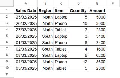
Suppose I want to import the following dataset into a new sheet, but only the rows where the Region (column 2) contains “South.” Instead of directly referencing column 2, I want to use a dynamic column ID so that the formula automatically adjusts if columns are inserted or deleted.

As mentioned earlier, we can make the column reference dynamic in QUERY IMPORTRANGE using Named Ranges. Here’s how.

Steps in the Source Sheet:

1. Select the range A1:E.
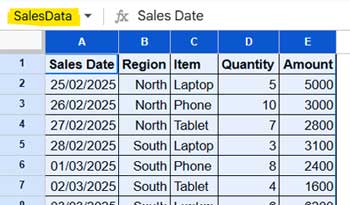
2. In the Name Box (top-left, next to the formula bar), you’ll see A:E.
3. Click the Name Box and type a name for this range, e.g., SalesData.
   
4. Navigate to an empty cell outside the data range, e.g., H1.
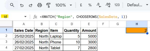
5. Enter the following formula to calculate the dynamic column ID of the Region column:
   =XMATCH("Region", CHOOSEROWS(SalesData, 1))
   • This formula searches for the field label “Region” in the first row of the named range and returns its position.
6. Click the Name Box again and name this cell id.

At this point, we have created two named ranges in the source sheet:

• SalesData (for the full dataset)
• id (for the dynamic column number)

To avoid accidentally deleting the helper cell H1, consider filling it with a distinct color to make it stand out.

Steps in the Destination Sheet:

1. In cell A1 of the destination sheet, enter the following formula to import the dynamic column identifier:
   =IMPORTRANGE("https://docs.google.com/spreadsheets/d/1I62hdJ0mK5WhgXdoMWBfcAd-fFmN2KbwbSgdcNK2mes/edit?gid=0", "id")
2. When prompted, click Allow Access.
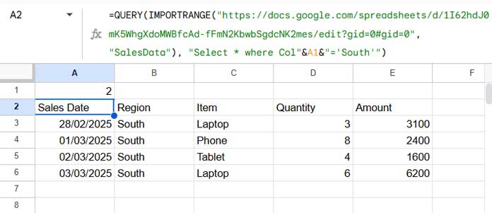
3. In cell A2, enter the following QUERY IMPORTRANGE formula:
   =QUERY(IMPORTRANGE("https://docs.google.com/spreadsheets/d/1I62hdJ0mK5WhgXdoMWBfcAd-fFmN2KbwbSgdcNK2mes/edit?gid=0", "SalesData"), "Select * where Col2='South'")

Now, let’s modify the formula to use a dynamic column reference.

4. Replace Col2 with Col"&A1&", making the formula
   =QUERY(IMPORTRANGE("https://docs.google.com/spreadsheets/d/1I62hdJ0mK5WhgXdoMWBfcAd-fFmN2KbwbSgdcNK2mes/edit?gid=0", "SalesData"), "Select * where Col"&A1&"='South'")

Now, if columns are inserted, deleted, or moved to a different position, the formula will still reference the Region column dynamically. However, if the Region column itself is deleted, the formula will break.

Conclusion

That’s how you can specify a dynamic column ID in QUERY IMPORTRANGE using Named Ranges in Google Sheets. This method ensures that your QUERY function remains accurate even when columns shift within the source data.

Resources

• How to Use IMPORTRANGE with Conditions in Google Sheets
• How to Use QUERY with IMPORTRANGE in Google Sheets
• IMPORTRANGE Within FILTER Function in Google Sheets
• IMPORTRANGE Named Ranges in Google Sheets – A Complete Guide
• Dynamic Column in VLOOKUP IMPORTRANGE Formula in Google Sheets