The DVAR function is a database function in Google Sheets used to calculate the variance (a measure of variability) of a population sample.
Google Sheets offers different functions for calculating variance, depending on the type of data you have:
- Variance of the Whole Population (σ²): Use DVARP or the statistical functions VARP / VAR.P.
- Sample Variance (s²): Use DVAR or the statistical functions VAR / VAR.S.
Why Choose DVAR Over VAR/VAR.S?
Using DVAR can be more convenient when you want to apply criteria, as it allows for straightforward filtering. In contrast, if you wish to filter data with VAR / VAR.S, you will need to combine them with the FILTER function, which can complicate your calculations.
It’s important to note that variance is a critical component in calculating standard deviation.
- Sample Variance (s²) helps determine how far the values are dispersed from the mean.
- Sample Standard Deviation (s) estimates the amount of dispersion.
DVAR Function: Syntax Explained
Syntax:
DVAR(database, field, criteria)Arguments:
- database: The array/range of cells to use. It should be structured like a database table, with the first row containing labels (field names) for each column.
- field: The relative position of the column in the database or a text label corresponding to a column header. The function extracts values from this column for calculations.
- criteria: The conditions used to filter the array/range before calculation.
There are no optional arguments in this function.
Examples of the DVAR Database Function in Google Sheets
How do you use the DVAR function in Google Sheets? Here are some examples:
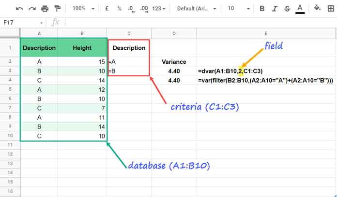
In column A, I have descriptions (A, B, and C) with multiple occurrences and their corresponding heights in column B.
For real-life relevance, you can replace these descriptions with cat breeds like “Persian,” “Maine Coon,” and “Bengal,” along with their respective heights in column B.
Example: Filter A and B and Calculate the Variance
The variance calculation formulas are in cells D3 and D4. In the D3 formula, I have used the relative position of 2 to apply the variance calculation to the “Height” column:
=DVAR(A1:B10, 2, C1:C3)Alternatively, you can use the field label “Height” itself:
=DVAR(A1:B10, "Height", C1:C3)
The following VAR formula alternative in cell D4 uses FILTER to exclude unwanted rows:
=VAR(FILTER(B2:B10, (A2:A10="A") + (A2:A10="B")))Can We Use the DVAR Function Without Criteria?
Yes! Here’s how to do it.
While all arguments in the function are mandatory, you can effectively use the DVAR function without specific criteria. When you want to include all values in the specified field column for variance estimation, you can use the following formula, where the criteria cover the entire column range:
=DVAR(A1:B10, 2, A1:A10)Unstructured Data and Virtual Field Labels
When you want to apply criteria in the variance calculation, the best option is to use the DVAR function. However, it requires structured data with proper field labels (a header row) at the top.
If you don’t have field labels, meaning you have a range rather than a database, you can follow this simple workaround.
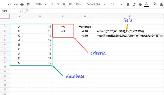
In the example below, there is no header row in the range for calculating variance. Since we can’t modify this, I have virtually added field labels by using blank entries:
=DVAR({"",""; A1:B10}, 2, {""; C2:C3})
Instead of specifying random names as row headers, I used blanks according to the number of columns in the ‘database’ (or range).
Conclusion
Do you know how the DVAR function treats blank cells and zeros in the evaluation column? In the example above, if any cells in column B are blank, the formula will ignore those rows. However, it will consider zeros, which may affect the results.
For further reading, you may find the following tutorials helpful in improving your skills with database functions in Google Sheets:


