


")


")

")
")
 in Excel & Google Sheets")


When you want to view a specific portion of a table, you can use the built-in Filter menu in Google Sheets. Alternatively, you can create your own drop-down to filter data from rows and columns, allowing you to extract data horizontally or vertically.
This method is particularly useful when you need to extract data into a new range for further analysis or calculations.
In this Google Sheets tutorial, I will show you how to create a drop-down menu to filter data dynamically—not just from rows but also from columns.
What’s more, I’ve also included a method to filter data both horizontally and vertically using a drop-down menu.
Below is a visual representation of what we will achieve in this tutorial:
1. Drop-Down Menu to Filter Rows in a Table
2. Drop-Down Menu to Filter Columns in a Table
3. Drop-Down to Filter Data From Rows and Columns
1. Drop-Down to Filter Data From Rows in Google Sheets
If you find the Filter command in Google Sheets limiting, you can use the FILTER function for more flexibility.
First, let me show you how to use a drop-down to filter data from rows. After that, we will move on to filtering columns and then combining both.
How to Create a Drop-Down Menu for Filtering Rows
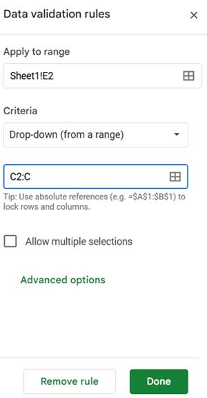
In the first example, the drop-down is in cell E2. Here’s how to create it:
- Navigate to cell E2.
- Click Insert > Drop-down.
- In the sidebar panel, select Criteria as Drop-down (from a range).
- Enter the range C2:C.
- Click Done.
Even if there are duplicate values in the range, Google Sheets will automatically ensure that only unique values appear in the drop-down menu.
Now, your drop-down to filter data from rows is ready. Use this FILTER formula in E3:
=FILTER(A2:C, C2:C=E2)2. Drop-Down to Filter Data From Columns in Google Sheets
Now, let’s filter columns dynamically by searching for a specific header. The goal is to extract data from the column that matches the selected header.
How to Create a Drop-Down Menu for Filtering Columns
The drop-down for column filtering is in G1. Follow the same steps as before to create the drop-down, but this time, enter the range B1:E1 (instead of C2:C), as we want to list unique headers in the drop-down.
For filtering columns, instead of using the FILTER function, we will use the INDEX-MATCH combination, as it allows us to extract data based on the selected column header.
Use this formula in G2:
=INDEX(A2:E, 0, MATCH(G1, A1:E1, 0))This formula looks for the header in G1, finds its position, and returns the corresponding column’s data.
Note: If you have duplicate headers—which is rare in structured data—you should consider using the FILTER function instead. Here’s the formula:
=FILTER(A2:E, A1:E1=G1)This formula extracts all columns where the header matches G1, making it useful when duplicate headers exist.
3. Drop-Down to Filter Data From Rows and Columns in Google Sheets
The third example combines both of the above techniques. We will use two drop-down menus—one to filter rows and the other to filter columns.
- H4: Drop-down menu to filter rows (created from range A4:A).
- H6: Drop-down menu to filter columns (created from range C3:F3).
Now, let’s filter the table using a single formula in J4:
=FILTER(FILTER(A3:F, (A3:F3=H6)+(A3:F3="Name")+(A3:F3="Exam")), A3:A=H4)Explanation:
- The inner FILTER extracts columns based on the selected value in H6.
- It also ensures that the “Name” and “Exam” columns are always included. The “Name” column is necessary for row filtering, but you can remove the “Exam” column if it’s not needed:
+(A3:F3="Exam")
This approach offers an efficient way to use drop-downs to filter data from rows and columns in Google Sheets.
Alternative Approaches
There are multiple ways to filter data both vertically and horizontally. The method above is one approach, but you may also find the following tutorials helpful:
Related Resources:
- Two-Way Filter in Google Sheets: Vertical & Horizontal
- How to Perform Two-Way Lookup Using VLOOKUP in Google Sheets
- Two-Way Lookup and Return Multiple Columns in Google Sheets
- Two-Way Lookup with XLOOKUP in Google Sheets
- Filter Data Using a Multi-Select Drop-Down in Google Sheets
- Filter Rows Containing Multiple Selected Values in Google Sheets
Download the sample Google Sheet used in this tutorial to practice on your own.
If only you had a video for these tutorials it would be useful. But I see no video.