Creating an in-cell drop-down menu from a single array is straightforward in Google Sheets using Data Validation. But what if you want to create a drop-down menu from multiple ranges?

Whether your values are static (unchanging) or dynamic (expanding over time), the method you use may vary slightly. In this tutorial, I’ll cover both cases to show you how to create a drop-down menu from multiple ranges in Google Sheets effectively.

Basic Drop-Down Menu From a Single Range

Before jumping into multiple ranges, let’s quickly revisit how to create a basic in-cell drop-down menu.

In the range C2:C11, I have numbers 1 to 10. I want to use these values to create a drop-down menu in cell A2.

Steps:

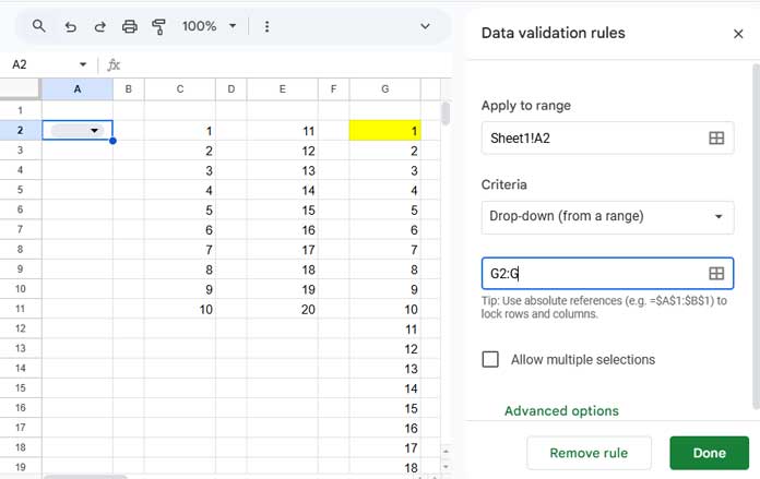
1. Click on cell A2, then go to Insert > Drop-down.
2. Under Criteria, choose Drop-down (from a range).
3. In the range field below, enter C2:C11 and click Done.

This sets up a standard drop-down menu using a single range.

How to Create a Drop-Down Menu From Multiple Ranges

Now, let’s talk about the actual topic—creating a drop-down menu from multiple ranges in Google Sheets.

Suppose:

• Range C2:C11 contains numbers 1 to 10.
• Range E2:E11 contains numbers 11 to 20.

Together, these make a complete list from 1 to 20, but they’re located in separate columns. You’ll need to combine them into a single column to use them in a drop-down menu.

Combine Multiple Ranges for Data Validation

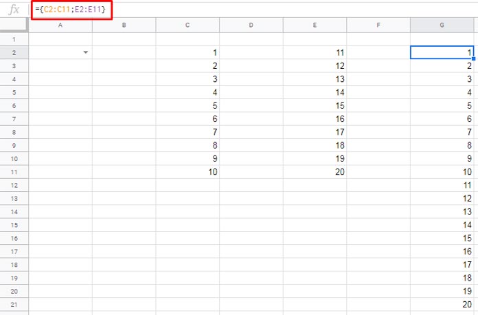
Use one of the following formulas in a helper column (for example, starting in cell G2) to stack these values:

={C2:C11; E2:E11}

Or, using VSTACK:

=VSTACK(C2:C11, E2:E11)

This vertically stacks the two column ranges into a single column, which can then be used in a drop-down menu.

You can even use data from different sheets within the same file. Just specify the sheet name along with the range, like this:

={Sheet1!C2:C11; Sheet2!E2:E11}

This combines values from multiple sheets into one list, which you can then use as the source for your drop-down menu.

Creating a Dynamic Drop-Down Menu From Multiple Expanding Ranges

If your source ranges are likely to grow (i.e., new values may be added later), use the TOCOL function to make the drop-down list dynamic:

=TOCOL({C2:C, E2:E}, 1, TRUE)

or

=TOCOL(VSTACK(C2:C, E2:E), 1, TRUE)

Once you enter this formula (say, in G2), select the output range (like G2:G) in the Drop-down (from a range) field when setting up Data Validation.

This approach automatically includes new values added to either C:C or E:E in the drop-down.

Can You Use More Than Two Ranges?

Absolutely! You can create a drop-down menu from three or more ranges the same way—just expand your formula:

=TOCOL({C2:C, E2:E, F2:F}, 1, TRUE)

Or

=TOCOL(VSTACK(C2:C, E2:E, F2:F), 1, TRUE)

The key is to vertically stack all values you want to appear in the drop-down menu, even if they’re from non-adjacent ranges.

Summary

Creating a drop-down menu from multiple ranges isn’t a built-in feature, but with a small helper formula, you can make it work dynamically and elegantly. This is perfect for maintaining cleaner Sheets, especially when your options are spread across different areas.

Related Reading

• Display Data from Any Sheet with Google Sheets Dropdowns
• Google Sheets: Add an ‘All’ Option to a Drop-down from Range
• Populate an Entire Month’s Dates Based on a Drop-down in Google Sheets
• Create a Drop-Down for Filtering Rows and Columns
• Multi-Row Dynamic Dependent Drop-Down List in Google Sheets
• Auto-Populate Information Based on Drop-down Selection in Google Sheets
• Distinct Values in Drop-Down List in Google Sheets
• How to Prevent Duplicates in Google Sheets
• The Best Data Validation Examples in Google Sheets