This tutorial explains how to create custom time slot sequences in Google Sheets using modern functions, such as XLOOKUP, MAKEARRAY, TOCOL, and SEQUENCE. You will also get a named function to simplify things.
No matter what your needs are, creating a date sequence with custom time slots in Google Sheets is a simple and effective way to keep track of your time and stay organized.
For example, if you have 5 time slots per day for event signups for a week, you can use my formula to create the sequence and use checkboxes in the next column to indicate the signups.
As a side note, if you want to book slots based on days or nights, you might try my popular reservation and booking calendar template, which is free, visually appealing, and features bars.
I assume your requirements may vary, so I am providing three different custom time slot sequence formulas:
- Only time slot sequence (array formula)
- Plus a date sequence in the next column (array formula)
- Both are in one column similar to timestamps (array formula)
Custom Time Slot Sequence Array Formula in Google Sheets
Example
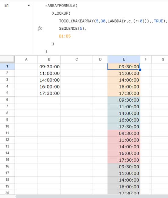
In the following example, I use 5 custom time slots (in cell range B1:B5) per day and want to use them for 30 days. You can use any number of time slots and days, and I will tell you how to modify the formula.
Formula
Enter the following formula in any cell in an empty column:
=ARRAYFORMULA(
   XLOOKUP(
      TOCOL(MAKEARRAY(5,30,LAMBDA(r,c,(r+0))),,TRUE),
      SEQUENCE(5),
      B1:B5
   )
)
Note: Select the result range and then click Format > Number > Time.

Explanation
This formula will populate a custom time slot sequence with your five provided time intervals for 30 days. There will be values in 150 (30 * 5) rows.
Breakdown
The formula is essentially an XLOOKUP formula that uses the first three arguments:
TOCOL(MAKEARRAY(5, 30, LAMBDA(r, c, r + 0)))is thesearch_key.SEQUENCE(5)is thelookup_range.B1:B5is theresult_range.
Here is a breakdown of each argument:
search_key
The search_key is a sequence of numbers in 5 rows and 30 columns. The MAKEARRAY function creates a matrix with 5 rows and 30 columns, with each value in the array equal to the row number.

The TOCOL function converts the sequence to a single column in the order {1, 2, 3, 4, 5, 1, 2, 3, 4, 5, …}.
lookup_range
The lookup_range is a sequence of numbers from 1 to 5. The SEQUENCE function creates this sequence.
result_range
The result_range is the cell range containing the time slots.
The XLOOKUP function searches for the search_key in the lookup_range and returns the corresponding values from the result_range. This allows us to repeat the set of time intervals 30 times.
How to Modify the Formula
To modify the formula for a different number of time slots per day and occurrences, simply change the values in the MAKEARRAY function and the SEQUENCE function. For example, to create a time slot sequence with 7 time intervals (B1:B7) per day for 10 days, you would use the following formula:
=ARRAYFORMULA(
   XLOOKUP(
      TOCOL(MAKEARRAY(7,10,LAMBDA(r,c,(r+0))),,TRUE),
      SEQUENCE(7),
      B1:B7
   )
)
Create Custom Time Slot Sequences with Independent Date Sequence in Google Sheets
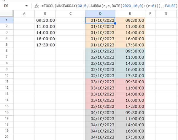
In our example above, we created a custom time slot sequence in the range E1:E. How about adding a corresponding date sequence in the range D1:D?
This is not a complex task. We can copy the XLOOKUP search key, which is the TOCOL + MAKEARRAY combination, and make a minor modification to it.
Here is the search key used in our earlier formula:
TOCOL(MAKEARRAY(5, 30, LAMBDA(r, c, r + 0)))In this, we should make two changes:
- replace 5 with 30 and 30 with 5.
- Replace the formula
r + 0withDATE(2023,10,1)-1+(r+0).
I want to start the dates from 1 Oct 2023. So the year in the DATE part of the formula is 2023, the month is 10, and the day is 1.
Here is the updated formula:
=TOCOL(MAKEARRAY(30,5,LAMBDA(r,c,DATE(2023,10,1)-1+(r+0))),,FALSE)In cell D1, insert the above array formula (make sure that D1:D has no value or formula beforehand).

Note: Select the result range and then click Format > Number > Date.
Create Date Sequences with Custom Time Slots in DateTime Format in Google Sheets
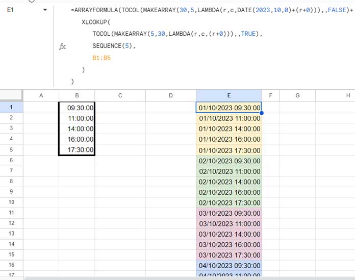
We have already seen array formulas to create a custom slot sequence and an additional date sequence column. To create a date sequence with a custom time slot sequence in the datetime or timestamp format, simply combine the two formulas within the ARRAYFORMULA function.
Below is an example of how to do this, using two different colors for each formula to make it easier to understand:
=ARRAYFORMULA(
   TOCOL(MAKEARRAY(30,5,LAMBDA(r,c,DATE(2023,10,1)-1+(r+0))),,FALSE)+
   XLOOKUP(
      TOCOL(MAKEARRAY(5,30,LAMBDA(r,c,(r+0))),,TRUE),
      SEQUENCE(5),
      B1:B5
   )
)
Key:
- Red: Time slot sequence
- Purple: Corresponding date sequence
Note: Select the result range and then click Format > Number > Date time.

Create Dynamic Custom Time Slot Sequence with the CUSTOMTIMESLOTS Named Function
I’ve provided three different array formula solutions to create custom time slot sequences in Google Sheets. I’m sure you’ll like the last formula that returns the output in datetime format.
However, you may find it difficult to use when you want to specify a different set of time intervals and occurrences, because you need to modify arguments in many parts of the formula. Let’s solve this problem with a dynamic formula and a named function.
Dynamic Formula
To make it dynamic, you just need to specify the range containing the time intervals you want in the sequence, how many times to repeat the time intervals, and the start date, you can use the following formula:
=LET(
   range,B1:B5,
   n,30,
   start_date,DATE(2023,10,1),
   ARRAYFORMULA(TOCOL(MAKEARRAY(n,COUNTA(TOCOL(range,1)),
   LAMBDA(r,c,start_date-1+(r+0))),,FALSE)+
   XLOOKUP(TOCOL(MAKEARRAY(COUNTA(TOCOL(range,1)),n,
   LAMBDA(r,c,(r+0))),,TRUE),SEQUENCE(COUNTA(TOCOL(range,1))),
   TOCOL(range,1)))
)
You need to specify three arguments:
range: The range containing the custom time slots (time intervals) to repeat. You can specify B1:B5 or B1:B to make it dynamic.n: The number of times to repeat each set of time slots. It’s 30 in our example above.start_date: The date to start the sequence, which is October 1, 2023.
CUSTOMTIMESLOTS Named Function in Google Sheets
The CUSTOMTIMESLOTS named function is a Google Sheets function that creates a dynamic custom time slot sequence. You can import it from my sample sheet below:
The CUSTOMTIMESLOTS function is useful for creating dynamic time slot sequences for a variety of purposes, such as scheduling appointments, managing resources, or tracking events.
Syntax and Arguments:
CUSTOMTIMESLOTS(range, n, start_date)Arguments:
range: The range containing the custom time slots (time intervals) to repeat.n: The number of times to repeat each time slot.start_date: The date to start the sequence.
The function returns an array of datetime values, representing the sequence of time slots.
Here is a short example of how to use the CUSTOMTIMESLOTS function:
=CUSTOMTIMESLOTS(B2:B5,4,DATE(2023,10,22))This formula will create a sequence of 4 time slots, starting on October 22, 2023.
Note: Select the result range and then click Format > Number > Date time.
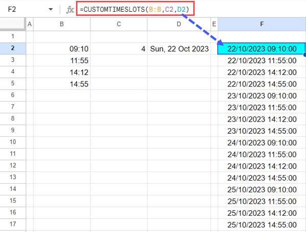
If you prefer cell references as inputs, use them as shown below:
=CUSTOMTIMESLOTS(B:B,C2,D2)
The CUSTOMTIMESLOTS function is a powerful tool for creating dynamic time slot sequences in Google Sheets.
Related: How to Count Events in Particular Timeslots in Google Sheets.


