Counting values across multiple columns row by row in Google Sheets can be tricky, especially if you want to do it efficiently without writing separate formulas for each row. Luckily, with an array formula combined with COUNTIF, you can automate this process and save a lot of time.

In this tutorial, we’ll walk you step by step through how to count occurrences across columns for each row, provide practical examples, and even share tips for customizing the formula to suit your data.

We will start with the traditional drag-down formula first and then move on to array formulas using BYROW and a classic DCOUNT workaround. Lots of interesting things for you to learn!

1. COUNTIF Across Columns Row by Row – Drag-Down

In the following example, we have test scores in columns A to E with field labels in the first row.

Assume you want to count scores greater than or equal to 10. You can use this COUNTIF formula in cell F2 and drag it down as far as you want:

=COUNTIF(A2:E2, ">=10")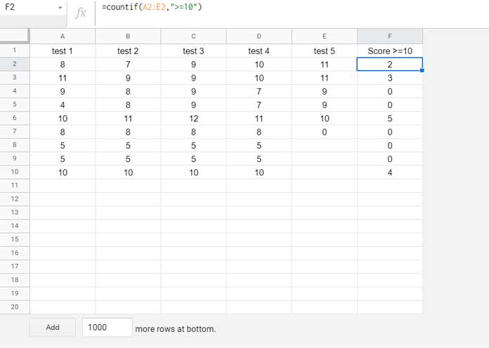

Note for Beginners

Enter the formula in F2, then either copy (Right Click → Copy) and paste (Right Click → Paste) in the rows below, or click and drag the fill handle (small blue circle at the bottom-right corner of F2).

This way you can get the count results across columns row by row in Google Sheets.

2. COUNTIF Across Columns Row by Row Using Array Formulas

You cannot use ARRAYFORMULA directly to expand the above COUNTIF across multiple rows since COUNTIF applies a single criterion to a range.

For example:

=COUNTIF(A2:E10, ">=10")

returns the count in the entire range, and

=ARRAYFORMULA(COUNTIF(A2:E10, ">=10"))

returns the same single result.

So a better solution is to use BYROW to apply COUNTIF row by row.

2.1 BYROW with COUNTIF Across Columns Row by Row

We can now expand a COUNTIF formula to conditionally count values across columns row by row using BYROW in Google Sheets.

Enter the following formula in cell F2:

=BYROW(A2:E, LAMBDA(r, IF(COUNTA(r)=0,, COUNTIF(r, ">=10"))))

It will populate values in F2:F.

Formula Explanation

Base non-array formula:

=COUNTIF(A2:E2, ">=10")

Array formula using BYROW and LAMBDA:

=BYROW(A2:E, LAMBDA(r, COUNTIF(r, ">=10")))

• The above formula returns 0 in blank rows.
• To return blank instead of 0, we use IF(COUNTA(r)=0,, …).

2.2 DCOUNT Alternative – Classic Formula

This is one of the approaches I was using to conditionally count values across columns row by row before the introduction of LAMBDA functions in Google Sheets.

Enter this formula in cell F2:

=ARRAYFORMULA(IFERROR(1/
   DCOUNT(
      TRANSPOSE({ROW(A2:A), IF(A2:E>=10, A2:E, )}), 
      SEQUENCE(ROWS(A2:A)), 
      {IF(,,); IF(,,)}
   )^-1
))

Note:

• If the count is 0, it will return an empty cell.

DCOUNT Formula Logic

DCOUNT Syntax:

DCOUNT(database, field, criteria)

We can use the DCOUNT function to count values in each column. By default, it counts column-wise, not row by row.

Example without any condition:

=ARRAYFORMULA(
   DCOUNT(
      A1:E10, 
      {1,2,3,4,5}, 
      {IF(,,); IF(,,)}
   )
)

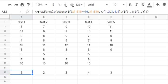
To apply a condition, for instance >=10, we can use a logical test within the database:

=ARRAYFORMULA(
   DCOUNT(
      IF(A1:E10>=10, A1:E10,), 
      {1,2,3,4,5}, {IF(,,); 
      IF(,,)}
   )
)

DCOUNT Across Multiple Columns

If you understand conditional column counting, you can see how to use DCOUNT in Google Sheets as a precursor to COUNTIF across columns row by row.

• Transpose the range A2:E10 (not A1:E10).
• Since A1:E1 contains field labels, we must use virtual field labels so DCOUNT can work correctly (it’s a database-based function and requires labels).

Formula components:

• data → TRANSPOSE({ROW(A2:A), IF(A2:E>=10, A2:E, )})
• index → SEQUENCE(ROWS(A2:A))
• criteria → {IF(,,); IF(,,)}

Using:

=ARRAYFORMULA(IFERROR(1/...^-1))

ensures that any zero counts are displayed as blanks, effectively removing zeros from the result.

Sample Sheet

Copy Sample Sheet

Resources

• Expand Count Results in Google Sheets
• Row-Wise COUNTUNIQUEIFS in Google Sheets (Array Formula)
• Count Empty or Blank Cells in Rows in Google Sheets
• Get the Count of Occurrences in Each Row in Google Sheets