


")


")

")
")
 in Excel & Google Sheets")


Need to get the count of occurrences of each value in a column—row by row? In other words, you want a reverse running count of items in Google Sheets.
In this tutorial, you’ll learn two approaches:
- A simple COUNTIF formula you can drag down
- A dynamic array formula that works without manual updates
Both help you track how often each value appears after its current row—great for cleaning duplicates or analyzing repeat entries.
Sample Data and Use Case
Suppose your data is in B2:B11 with repeated names. You want to count how many times each name appears from that row downward.
Method 1: COUNTIF to Get the Count of Occurrences (Non-Array Formula)
Formula in C2:
=COUNTIF(B2:B11, B2)Then drag it down. Each row updates automatically:
- In C3 →
=COUNTIF(B3:B11, B3) - In C4 →
=COUNTIF(B4:B11, B4)
Limitations:
- You must extend or copy the formula when adding new rows.
- Inserting rows mid-range breaks the continuity.
Method 2: Reverse Running Count with Array Formula
For a fully automated solution, use this array formula:
=ArrayFormula(COUNTIFS(B2:B11, B2:B11, ROW(B2:B11), ">="&ROW(B2:B11)))This counts how many times each value appears from its row to the end of the range.
Why It’s Called a Reverse Running Count
- Top-down: It counts how often the item appears from that point forward.
- Bottom-up: It resembles a traditional running count, in reverse.
Cleaner Version for Dynamic Ranges
To handle longer datasets without trailing zeros:
=ArrayFormula(
  LET(
    reverseRc, COUNTIFS(B2:B, B2:B, ROW(B2:B), ">="&ROW(B2:B)),
    IF(reverseRc, reverseRc, "")
  )
)
This version uses LET to define a name for the intermediate result and IF to blank out any zero counts.
Formula Explanation
=ArrayFormula(
  LET(
    reverseRc, COUNTIFS(B2:B, B2:B, ROW(B2:B), ">="&ROW(B2:B)),
    IF(reverseRc, reverseRc, "")
  )
)
What it does:
COUNTIFS(...): Counts how many times each value appears from that row downward.LET(...): Defines a variable (reverseRc) to hold the result.IF(...): Removes zero counts from blank rows by replacing them with empty strings.
When to Use Each Method
| Use Case | Method |
|---|---|
| You prefer copy-pasting formulas | COUNTIF Drag Formula |
| You want a clean, auto-updating result | Array Formula with LET |
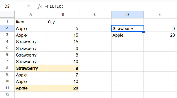
Real-Life Use: Filter Latest Records
Let’s say your dataset is in chronological order, but you don’t have timestamps. The last occurrence of a value in the column indicates the most recent record.
To extract only the latest entries:
=FILTER(
   A2:B,
   LET(
      reverseRc, COUNTIFS(A2:A, A2:A, ROW(A2:A), ">="&ROW(A2:A)),
      IF(reverseRc, reverseRc, "")
   )=1
)
This filters rows where the reverse running count is 1—i.e., the last time that value appears.
Alternatively, you can use SORTN:
=SORTN(SORT(A2:B, ROW(A2:A)*(A2:A<>""), FALSE), 9^9, 2, 1, TRUE)But keep in mind:
SORTNmay reorder dataFILTERpreserves original order
FAQ
Q: What’s a reverse running count?
A: It’s the count of how many times each value appears from its current row to the bottom of the column.
Q: How is it different from a regular running count?
A: A regular running count counts upward from the start of the range, while a reverse running count looks downward.
Q: Can I use this with open-ended ranges like B2:B?
A: Yes! The optimized formula using LET handles open-ended ranges and removes trailing 0s.
Q: Will the array formula auto-update with new rows?
A: Yes, as long as you’re using open-ended ranges like B2:B, the formula will adapt automatically.
Resources
Explore related guides for variations and extensions:
- Running Count in Google Sheets: Formula Examples
- Case-Sensitive Running Count in Google Sheets
- Cumulative Count of Distinct Values in Google Sheets
- Fix Interchanged Names in Running Count in Google Sheets
- Reverse an Array in Google Sheets
- FLIP in Google Sheets – Custom Named Function to Reverse Data
- Reverse Running Total in Google Sheets (Array Formula)
Hi Prashanth,
May I get the formula for the same without the reversing? I would like to get 1,2,3.. instead of reverse order.
Thanks,
Saravanan N K
Hi, Saravanan N k,
Replace B2:B with your actual range.
=ArrayFormula(let(rc,COUNTIFS(B2:B,B2:B,ROW(B2:B),"<="&ROW(B2:B)),if(rc=0,,rc)))Prashanth,
Not sure what you’re trying to get with your arrayformula.
Have you tried;
1) either us relative/absolute markers in your formulas? Dragging or copy/pasting will actually work if you use a simple
=COUNTIF($D$26:$D$33;$D26)2) or use a very simple Arrayfomula such as
=ARRAYFORMULA(COUNTIF(D26:D33;D26:D33))Both give the same result, and are not too complex 🙂
Hi, Frank Oers,
The difference in cumulative aka running count.
If an item, for example, “book” repeated 5 times, in each row your formula would return 5. But mine would 1, 2,…5.