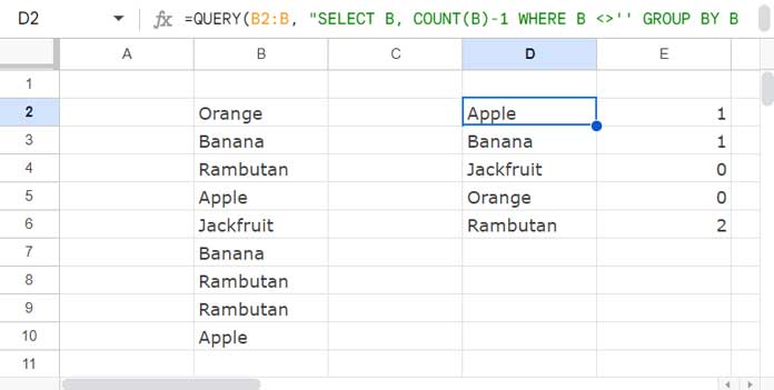
How to Count Duplicate Values in a Column in Google Sheets

We can use either a QUERY or a UNIQUE and COUNTIF combo to count duplicate values in a column in Google Sheets. Both solutions will work whether you want to include or exclude the first occurrence.

Highlighting is one option to identify duplicate values in a column. However, when your dataset is very large, it may affect the performance of the Sheet.

Alternatively, the formula creates a new list with unique values and shows how many times each duplicate value is present. This helps you track duplicates very easily because you can then apply a FILTER to those values and delete or highlight whatever you want.

Counting Duplicate Values Using the QUERY Function

The values to count for duplicates are in B2:B.

The following QUERY formula will count duplicate values excluding the first occurrence in column B:

=QUERY(B2:B, "SELECT B, COUNT(B)-1 WHERE B <>'' GROUP BY B LABEL COUNT(B)-1''", 0)

Counting Duplicate Values Using the QUERY Function

If you want to get the count including the first occurrence, simply replace COUNT(B)-1 with COUNT(B) in both the SELECT and LABEL clauses of the query.

The QUERY function selects column B and COUNT(B)-1, then filters the rows where column B is not null and groups column B. The LABEL clause removes the header label.

The formula will automatically include new values since the range is open, which is B2:B, not B2:B10.

Counting Duplicate Values Using the UNIQUE and COUNTIF Combo

First, we will get unique values from B2:B using the following UNIQUE formula in cell D2:

=UNIQUE(B2:B)

Then, in cell E2, enter the following COUNTIF formula to count corresponding duplicate values in the list:

=ArrayFormula(COUNTIF(B2:B, D2:D6)-1)

Where B2:B is the range to count and D2:D6 is the criteria to test against the range.

This formula has one drawback: the range is open, but the criteria (the UNIQUE result range) is not open.

Do you want to use this formula similarly to QUERY?

Let’s combine these UNIQUE and COUNTIF functions into a single formula and also open the range in both. Here you go:

=ArrayFormula(LET(list, B2:B, ulist, TOCOL(UNIQUE(list), 1), HSTACK(ulist, COUNTIF(list, ulist)-1)))

I’ve utilized the LET function to assign names to value expressions and use them in the subsequent calculation.

When you use this, simply replace B2:B with the column from which you want to count the duplicates.

Similar to QUERY, if you want to return the count of duplicates including the first occurrence, remove -1 in the formula.

FAQs

How to count duplicate values in more than one column?

Assume you have data in columns A and B, for example, A2:B. In the above formulas, replace B2:B with TOCOL(A2:B, 1).

In addition, in QUERY, you should replace the column identifier B with Col1 wherever it appears.

Can I get the duplicate count alongside the original values?

Yes. In our example, the range is B2:B. In cell C2, you can enter the following formula to get the duplicate count:

=ArrayFormula(IF(B2:B="",,COUNTIF(B2:B, B2:B)-1))

Do these formulas work in Excel?

No, they do not. They are specifically coded for Google Sheets.