We can use a combination of formulas to count a specific character in Google Sheets. The particular characters can be alphabets (case sensitive or case insensitive), numbers, or special characters such as a pipe, tilde, whitespace, newline, etc.

I have two types of combinations (formulas) for this. One uses regular expressions, and the other does not use any regular expressions.

Both formulas have one thing in common: they use the LEN function. The good thing is that the latter one will also work in Excel.

So, whether you are a Google Sheets or Excel user, you can use my formula for your specific needs.

Count the Occurrence of a Specific Character in a Cell

Let’s start with the first combination formula, which uses SUBSTITUTE and LEN, as it will work in both of the two popular spreadsheet applications – Excel and Google Sheets.

Option 1: Using SUBSTITUTE and LEN

To count the total number of characters in a string, there is a function called LEN in Google Sheets/Excel.

Let’s see how to use the SUBSTITUTE and LEN combination to count a specific character in Google Sheets.

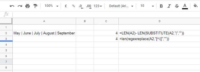
Cell A2 contains the following string:

May | June | July | August | September

I want to count the number of “|” characters, which are the separators in the said string. Here are the steps.

Using the following LEN function, we can get the total number of characters in cell A2. Here it would be 38.

=LEN(A2) // returns 38

Now, what we want to do is SUBSTITUTE the character “|” with null and get the length of characters using the following formula.

=LEN(SUBSTITUTE(A2, "|", "") // returns 34

It would return 34. So the count of the said character will be 38 – 34 = 4. We can write the combination formula as below.

=LEN(A2)- LEN(SUBSTITUTE(A2, "|", "")) // returns 4

Option 2: Using REGEXREPLACE and LEN

Instead of replacing the specific character, we will replace all the other characters in the string using REGEXREPLACE and count the remaining characters using LEN.

=LEN(REGEXREPLACE(A2, "[^\|]", ""))

Note: When counting a special character, escape them using \ (backslash character).

This formula won’t work in Excel.

Both of the above combination formulas are case-sensitive. To make them case insensitive, use the following formulas.

Case-Insensitive Formulas to Count a Specific Character in a Cell

Assume the text in cell A2 is “Abracadabra” and we want a case-insensitive count of the character “a” in this.

Both the following formulas will return 1 because they are case-sensitive.

=LEN(A2)- LEN(SUBSTITUTE(A2, "A", "")) // returns 1
=LEN(REGEXREPLACE(A2, "[^A]", "")) // returns 1

For a case-insensitive character count, follow this approach:

In the LEN and SUBSTITUTE combination, we can convert the cell value to lowercase and use the lowercase character to substitute.

=LEN(A2) - LEN(SUBSTITUTE(LOWER(A2), "a", "")) // returns 5

In the LEN and REGEXREPLACE combination, we can use the pattern (?i) as below.

=LEN(REGEXREPLACE(A2, "(?i)[^a]", "")) // returns 5

Count a Specific Character in a Range of Cells in Google Sheets

In all the above examples, we have counted a specific character in a particular cell, which is cell A2.

If you want to apply this to a cell range, for example, A2:B100, you can combine all the strings as follows:

TEXTJOIN("", TRUE, A2:B100)

The TEXTJOIN function combines all the strings in the range, leaving out blank cells.

Resources

• How to Count Comma Separated Words in a Cell in Google Sheets
• Count Words and Insert Equivalent Blank Rows in Google Sheets
• Split and Count Words in Google Sheets (Array Formula)
• Excel Word Count: Beyond SUBSTITUTE