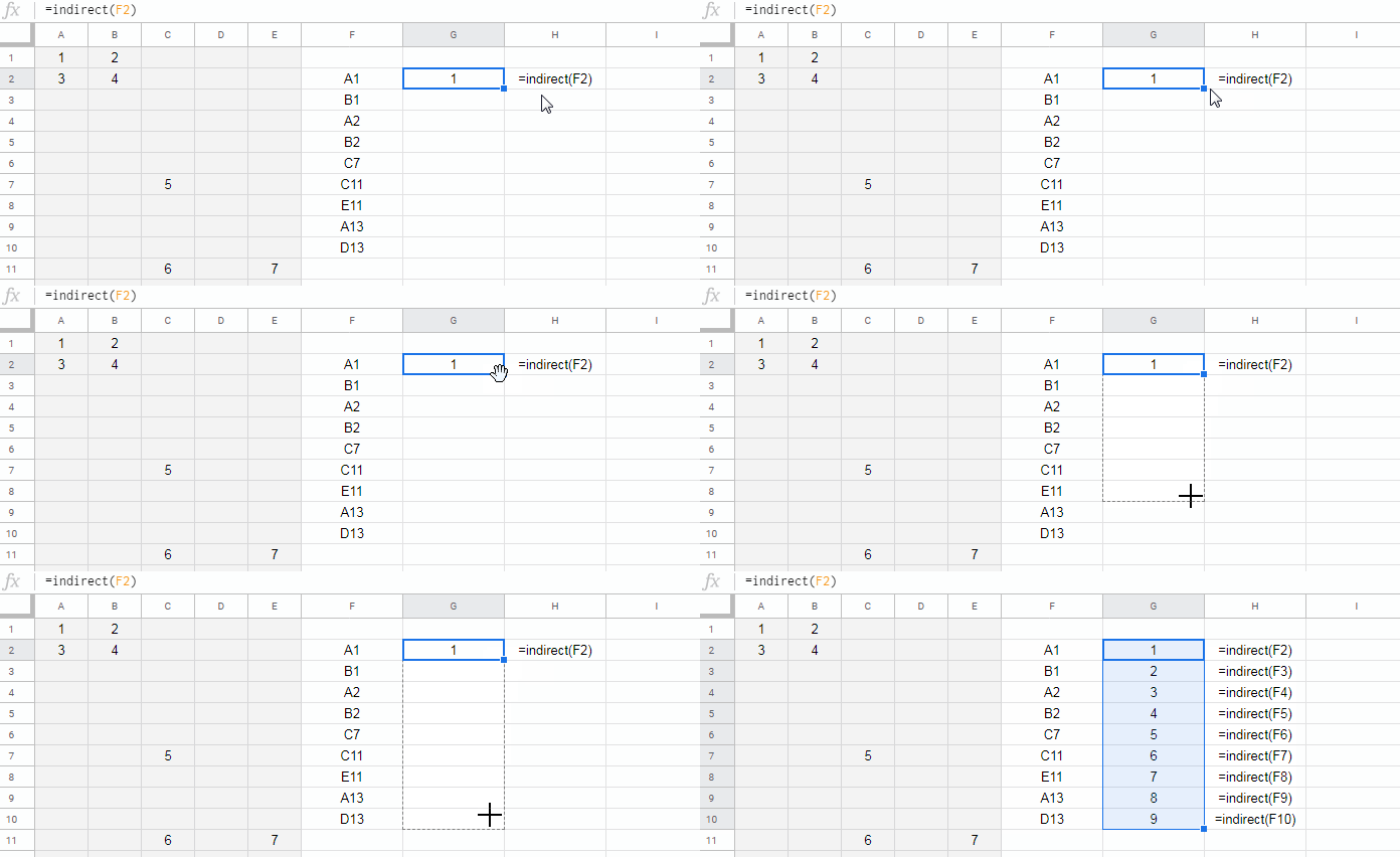
Sometimes in Google Sheets, you have a list of cell references like A1, B2, or C3, and you want to pull the actual values from those cells. Manually referencing each one can get tedious — especially when dealing with a larger range.

This is where an Array Formula comes in handy. In this tutorial, I’ll show you how to convert cell references to values with Array Formula in Google Sheets, so your workflow stays fast, flexible, and formula-driven.

Note: By “array formula,” I’m not referring to the ARRAYFORMULA function specifically, but to any formula that spills results across multiple cells.

Convert Cell References to Values – Non-Array Formula

To convert a cell reference to its value, you can use the INDIRECT function:

=INDIRECT("A1")

This will return the value from cell A1.

If you have a reference stored in a different cell — for example, if cell F2 contains "A1" — you can use:

=INDIRECT(F2)

That way, you can dynamically refer to different cells just by updating the content of F2.

Working with Multiple References

If you have a list of cell references, say in F2:F10, you can manually drag the formula down in a parallel column to fetch each value:

=INDIRECT(F2)
=INDIRECT(F3)
...

But this approach becomes messy and repetitive. Let’s fix that with an array solution.

Convert Cell References to Values – Array Formula

To convert a list of cell references to values all at once, we can use the MAP function with INDIRECT:

=MAP(F2:F10, LAMBDA(ref, INDIRECT(ref)))

Formula Breakdown

• F2:F10 is your list of cell references, like "A1", "B2", etc.
• LAMBDA(ref, INDIRECT(ref)) takes each reference from the range and converts it to its actual value.
• MAP applies the lambda function to each item in the list — returning the corresponding values in one go.

Note:
This formula may return a #REF! error if any cell in the reference range is empty or contains an invalid cell reference.
Additionally, if any reference in the range points to the same cell where the formula is applied, it will also result in a #REF! error due to a circular dependency. In such cases, the entire formula may break and fail to return any result.

To avoid these errors, you can wrap the formula with IFERROR:

=IFERROR(MAP(F2:F10, LAMBDA(ref, INDIRECT(ref))))

Example: MAP and INDIRECT with Cell References

Let’s say column F (F2:F4) has these values:

A1
A2
A3

And cells A1:A3 contain:

100
200
300

Using:

=MAP(F2:F4, LAMBDA(x, INDIRECT(x)))

…will return:

100
200
300

The results will spill into the same rows as the input range — so if the formula is entered in G2, the output will appear in G2:G4, aligned with F2:F4. No need to drag or copy the formula down manually.

FAQs

Can I convert a cell reference to value from another sheet in the same workbook?

Yes. Just include the sheet name in the reference.

For example, if F2 contains Sales Report!A1, the formula:

=INDIRECT(F2)

…will return the value in cell A1 of the Sales Report sheet.

Can I use ARRAYFORMULA instead of MAP?

No, INDIRECT is a bit tricky with ARRAYFORMULA, as it doesn’t natively expand across arrays. That’s why MAP (or alternatives like BYROW) is the better choice when working with ranges.

Does INDIRECT work with dynamic ranges?

Yes, but only when built correctly as a string. For example:

=INDIRECT("A"&ROW())

…will return the value in column A of the current row.

Conclusion

When you need to convert multiple cell references to their actual values in Google Sheets, INDIRECT does the job — but pairing it with MAP and LAMBDA makes it dynamic and scalable.

This technique is especially useful in dashboards, reports, and other scenarios where references are generated or pulled dynamically.

If you’re working with large data ranges and want to reduce manual steps, now you know how to convert cell references to values with Array Formula in Google Sheets — the clean, formula-first way.

Resources

• How to Freeze a Cell in IMPORTRANGE in Google Sheets (Lock a Cell Reference)
• Relative Cell Reference in IMPORTRANGE in Google Sheets
• How to Use Cell Reference in Google Sheets QUERY
• How to Use Cell Reference in Filter Menu (Filter by Condition) in Google Sheets
• Dynamic Cell Reference in Table of Contents in Google Sheets
• Drag Formula Right, Increment Cell Reference Down in Google Sheets
• Replace VLOOKUP and HLOOKUP with MATCH and INDIRECT in Google Sheets
• Highlight INDIRECT Range in Google Sheets
• Alternatives to INDIRECT with ArrayFormula in Google Sheets (Using LHFs)