


")


")

")
")
 in Excel & Google Sheets")


MMULT is primarily used for matrix multiplication, but it can also serve as an alternative to SUMPRODUCT to achieve similar results in a more expanded form. As a side note, SUMPRODUCT returns the sum of the products of corresponding entries in two equal-sized arrays or ranges, and we can apply specific conditions to control the sum of products. This is where the application of criteria or conditions in MMULT becomes important. Let’s explore how to perform conditional MMULT calculations to replace the SUMPRODUCT function in Google Sheets.
Understanding Conditional MMULT in Google Sheets
In the following example, I have items listed in A1:A7, their unit prices in B1:B7, and the monthly sales of these items from January to March across three columns (C1:E7).
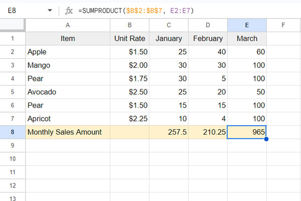
You can use the following SUMPRODUCT formula in cell C8 to calculate the total sales for January:
=SUMPRODUCT($B$2:$B$7, C2:C7)Drag this formula to E8 to get the total sales for the other months.
Alternatively, you can use the following MMULT formula in cell C8 to calculate the total sales for each month at once:
=MMULT(TRANSPOSE(B2:B7), C2:E7)This eliminates the need to drag the formula across multiple cells.
Now, let’s explore conditional MMULT with the same example.
Suppose you want to calculate the monthly sales for a specific item, such as “Pear.”
You can use the following SUMPRODUCT formula in cell C9 and drag it across:
=SUMPRODUCT($A$2:$A$7="Pear", $B$2:$B$7, C2:C7)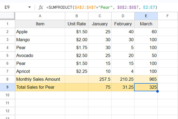
But how would you approach this using conditional MMULT?
Let’s dive into the details!
Example of Conditional MMULT in Google Sheets
The conditional MMULT formula is not much different from the regular MMULT formula mentioned above. What you need to do here is replace the unit rates of all other items with 0.
In our previous MMULT without criteria, the matrices are as follows:
- Matrix 1:
TRANSPOSE(B2:B7) - Matrix 2:
C2:E7
For the conditional version, Matrix 1 will be defined as IF(A2:A7="Pear", B2:B7, 0).
This logical test requires the ARRAYFORMULA, so you should enter the MMULT as an array formula.
Here is the conditional MMULT formula:
=ArrayFormula(MMULT(TRANSPOSE(IF(A2:A7="Pear", B2:B7, 0)), C2:E7))How Do We Specify Multiple Conditions?
Once you learn the above, specifying multiple conditions is not a Himalayan task.
For example, to get the total sales amount for the fruits “Pear” and “Avocado,” you can specify the conditions as follows:
Replace A2:A7="Pear" with (A2:A7="Pear")+(A2:A7="Avocado").
So, the conditional MMULT formula with multiple conditions will be:
=ARRAYFORMULA(MMULT(TRANSPOSE(IF((A2:A7="Pear")+(A2:A7="Avocado"), B2:B7, 0)), C2:E7))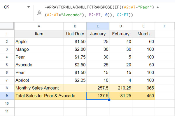
Additional Notes
Empty cells in matrix multiplication can cause errors in the formula. If you expect blank cells in any range (matrix 1 or matrix 2) specified in the formula, you should use the N function. The N function returns the value if it is not empty; otherwise, it returns 0.”
In the above examples, you can wrap B2:B7 (unit rates) and C2:E7 (quantities) with N as follows:
=ARRAYFORMULA(MMULT(TRANSPOSE(IF((A2:A7="Pear")+(A2:A7="Avocado"), N(B2:B7), 0)), N(C2:E7)))