You can use the following custom highlight rule to compare two Google Sheets tabs (worksheets) cell by cell and highlight cells with different values.

=A1<>(INDIRECT("Sheet2!"&ADDRESS(ROW(), COLUMN())))

The advantage of this formula is that it allows you to compare entire sheet tabs for differences or a specific range within both sheets. The latter is particularly useful when you want to compare two tables in separate sheets and is more performance-friendly.

I’ll explain how to use this formula rule in your sheet.

How to Compare Two Sheets in Google Sheets and Highlight Differences

Compare All Cells in Both Sheets for Highlighting

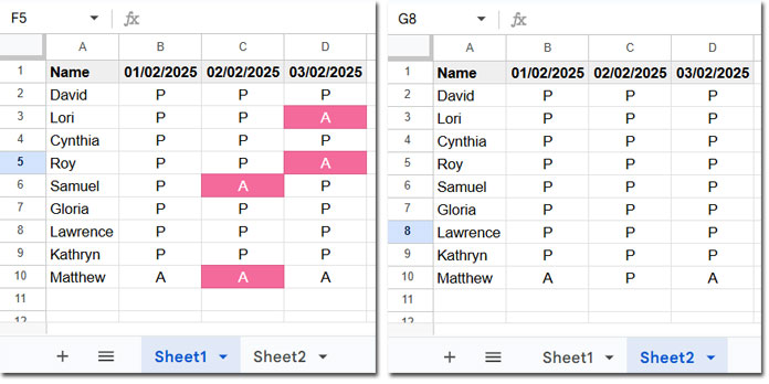
Let’s consider two sheets named Sheet1 and Sheet2 in a Google Sheets file.

To compare Sheet1 with Sheet2 and highlight cells where they don’t match in Sheet2:

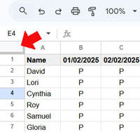
1. Select all cells in Sheet1. You can do this by clicking the blank square at the top-left corner of the grid, where the column letters and row numbers meet.
   
2. Then, click Format > Conditional Formatting.
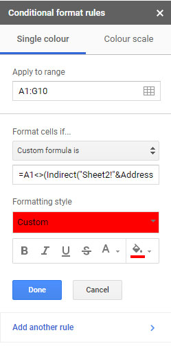
3. In the Conditional Format Rules panel on the sidebar, select Custom formula is under Format rules.
4. Enter the formula:
   =A1<>(INDIRECT("Sheet2!"&ADDRESS(ROW(), COLUMN())))
   Where Sheet2 refers to the sheet you are comparing with the active sheet (which you’re highlighting).
5. Choose a formatting style.
6. Click Done.

This will compare Sheet1 with Sheet2 and highlight the differences.

Note: You can follow the same steps in Sheet2 to compare it with Sheet1 and highlight the differences. The only difference is the formula. In that case, replace Sheet2 with Sheet1 in the formula.

Comparing a Specific Range in Both Sheets for Highlighting

Sometimes you may want to compare specific ranges, such as two tables with the same dimensions and located in the same range in two sheets.

For example, you may have one table in Sheet1 in the range B10:Z50, and another table in the same range in Sheet2.

To highlight the differences between these two ranges, follow these steps:

1. Select the range B10:Z50 by clicking B10, pressing the Shift key, and then clicking Z50.
2. Click Format > Conditional Formatting.
3. Select Custom Formula is.
4. Enter the formula:
   =B10<>(INDIRECT("Sheet2!"&ADDRESS(ROW(), COLUMN())))

Yes! The transformation is simple. In the formula, use the starting cell reference of the table.

What About Two Sheets in Two Workbooks?

If the sheets are in two different workbooks, use the IMPORTRANGE function to import one sheet into the second sheet. This way, both sheets will be in the same workbook.

After that, you won’t encounter any issues highlighting the differences by following the steps above.

Resources

• Compare Two Sheets in Google Sheets and Identify Differences
• How to Compare Two Columns for Matching Values in Google Sheets
• Compare Two Tables and Remove Duplicates in Google Sheets
• Google Sheets: Compare Two Lists and Extract Differences
• Compare Two Strings Irrespective of the Word Positions in Google Sheets
• Compare and Highlight Up and Down in Ranking in Google Sheets
• Compare Two Rows and Find Matches in Google Sheets
• How to Compare Comma-Separated Values in Google Sheets
• Compare All Columns with Each Other for Duplicates in Google Sheets
• Compare Two Tables for Differences in Excel