Want to build a code breaker game in Google Sheets using only formulas? In this tutorial, you’ll learn how to create a fully playable logic puzzle game without Apps Script.

This spreadsheet game works on both desktop and mobile devices. However, for the best setup and gameplay experience, I recommend using a desktop or laptop.

If you prefer not to build everything from scratch, you can also download the free template and start playing immediately.

What You’ll Build in This Code Breaker Game

In this tutorial, you’ll learn how to:

• Download and play the template.
• Build a code breaker game in Google Sheets from scratch.
• Generate a random hidden color sequence.
• Create automatic clue pegs using formulas.
• Display win/loss messages dynamically.

Download the Free Template

Get the ready-to-play Code Breaker Game for Google Sheets here:

Preview and Download

How to Play the Code Breaker Game in Google Sheets

In this puzzle, your goal is to discover a hidden sequence of four colors within 10 attempts.

Game Rules

1. Start from Row 1

Begin your first guess in Row 1 and continue downward until Row 10.

2. Choose Colors

In cells A:D, select one color in each cell until your guess is complete.

Available colors:

🟠 🔴 🟣 🟢 🟡 🔵

3. Read the Clues

After completing a row, clue pegs appear automatically.

• ⚫ = Correct color in the correct position
• ⚪ = Correct color in the wrong position
• ⬜ = Color not found in the hidden code

4. Make Your Next Guess

Use the clues to improve your next attempt.

Important: Clues show only the total matches. They do not reveal which positions are correct.

5. Win the Game

Find the hidden code before all 10 attempts are used.

6. Start a New Game

To generate a new hidden code and reset the game:

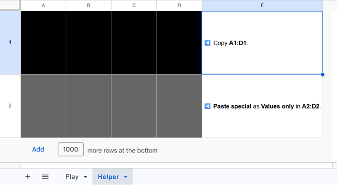
1. Open the Helper sheet.
2. Select the range A1:D1. These cells generate a new hidden color sequence as numeric character codes. Since the text color and background color are the same, the values remain hidden.
3. Copy the selected cells.
4. Select the range A2:D2.
5. Choose: Edit → Paste special → Values only
   Again, you won’t see the pasted values because these cells are also masked using the same text and background color.

This replaces the previous hidden code with a new one and starts a fresh game.

Important for Mobile Users:

The Google Sheets mobile app currently does not support Paste special → Values only for this setup.

To start a new game on mobile:

1. Open the spreadsheet link in your mobile browser instead of the app.
2. Sign in to your Google account if needed.
3. Open your browser menu and enable Desktop site.
4. Follow the same steps above to paste the new code as values only.

This gives you access to the full spreadsheet features required to reset the game.

For the smoothest gameplay and setup experience, I recommend using a desktop or laptop.

How to Create a Code Breaker Game in Google Sheets

Now let’s build the code breaker game in Google Sheets step by step.

1. Set Up the Play Area

Step 1: Create the Play Sheet

Create a new spreadsheet and rename the first sheet to:

Play

Step 2: Add Dropdown Colors

Select range:

A1:D10

Then choose:

Insert → Dropdown

Step 3: Configure Dropdown Rules

Add these dropdown values:

🟠
🔴
🟣
🟢
🟡
🔵

Under Advanced Options:

• Enable Reject input
• Set display style to Plain text

Step 4: Resize the Game Board

Set dimensions:

• Columns A:D = Width 40
• Rows 1:10 = Height 40

Step 5: Add Attempt Numbers

In cell E1, enter:

=SEQUENCE(10)

This generates attempt numbers from 1 to 10.

2. Create the Hidden Code

Add a second sheet named:

Helper

In cell A1, enter:

=BYCOL(SEQUENCE(1, 4), LAMBDA(r, INDEX({128992, 128308, 128995, 128994, 128993, 128309}, RANDBETWEEN(1, 6))))

This formula randomly generates four color codes.

Hide the Secret Code

• Format A1:D1 with a black background.
• Select A2:D2.
• Apply dark fill and dark text color.
• Copy A1:D1 and paste as Values only into A2:D2.

A2:D2 now stores the active hidden code used during gameplay.

3. Generate the Clues

In the Play sheet, enter this formula in cell F1:

=BYROW(A1:D10, LAMBDA(row, 
  LET(
     guess, row, 
     code, INDEX(CHAR(Helper!A2:D2)), 
     black, SUMPRODUCT(guess=code), 
     total_matches, SUM(MAP(UNIQUE(guess, TRUE), LAMBDA(c, IF(c="", 0, MIN(COUNTIF(guess, c), COUNTIF(code, c)))))), 
     white, total_matches - black, 
     IF(COUNTA(guess)<4,,REPT("⚫", black)&REPT("⚪", white)&REPT("⬜", 4-white-black))
  )
))

How This Formula Works

Counts exact matches (Black Pegs):

SUMPRODUCT(guess=code)

Counts all matching colors, regardless of position (Total Matches):

SUM(MAP(UNIQUE(guess,TRUE),LAMBDA(c,IF(c="",0,MIN(COUNTIF(guess,c),COUNTIF(code,c))))))

This prevents duplicate colors from being counted incorrectly.

White pegs are calculated as:

total_matches-black

4. Show Win or Loss Messages

In cell I2, enter:

=LET(
  win, IFNA(XMATCH("⚫⚫⚫⚫", F1:F10)), 
  IF(
    win, "🔓 You cracked the code in "&win&IF(win=1, " attempt", " attempts!"), 
    IF(
      AND(NOT(win), COUNTA(F1:F10)=10), "Loss: ❌ Game Over. The secret code was: "&JOIN("", INDEX(CHAR(Helper!A2:D2))),
    )
  )
)

This formula:

• Detects when all four positions are correct.
• Shows the number of attempts used.
• Reveals the hidden code if all attempts fail.

Final Thoughts

Building a code breaker game in Google Sheets is a fun way to explore interactive spreadsheet design using formulas alone.

Download the free template, test the game, and then customize it with your own colors, themes, or gameplay rules.

You May Also Enjoy

• Build a Sudoku Generator in Google Sheets
• Create a Snake and Ladder Game in Google Sheets
• Build a Word Guess Game in Google Sheets

Looking for more ready-to-use spreadsheet templates? Explore our Free Templates for Google Sheets (Fully Automated & Dynamic).