The AVERAGEIF function in Google Sheets allows you to calculate averages based on a specific condition applied to a row or column. This guide explains the syntax, provides examples, and offers practical tips.

For multiple conditions, you can use AVERAGEIFS, which supports more than one criterion. Let’s dive into the syntax and usage of the AVERAGEIF function in Google Sheets.

AVERAGEIF Function: Syntax and Arguments

Syntax:

AVERAGEIF(criteria_range, criterion, [average_range])

Arguments:

• criteria_range: The range to evaluate against the condition.
• criterion: The condition or pattern applied to criteria_range.
• average_range: The range of values to average. If omitted, criteria_range is used.

Examples

1. Average of values in B2:B100 where A2:A100 contains “Apple”:
   =AVERAGEIF(A2:A100, "Apple", B2:B100)
2. Average of values in B2:B100 where values are greater than 200:
   =AVERAGEIF(B2:B100, ">200")

Note: The AVERAGEIF function is case-insensitive.

Find Average Based on a Condition in Google Sheets

Here are some common use cases:

1. Using a Number as a Criterion

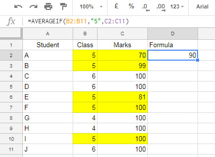
In the following example, A2:11, B2:B11, and C2:C11 contain student names, their class, and their marks, respectively.

To calculate the average marks scored by students in Class 5, use this formula:

=AVERAGEIF(B2:B11, 5, C2:C11)

You can also use double quotes for the criterion, such as "5". Google Sheets treats both 5 and "5" as equivalent when the criterion is a number.

For comparison operators (e.g., greater than or less than), numbers must be enclosed in quotes:

=AVERAGEIF(B2:B11, ">5", C2:C11)

2. Using Dates as a Criterion

Dates can be tricky due to formatting differences. To ensure accuracy in the conditional average calculation, use the DATE function or the ISO 8601 format (YYYY-MM-DD).

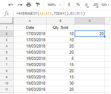
Sample Data: A2:A11 contains sales dates, and B2:B11 contains quantities sold.

• Average quantity sold on March 19, 2018:
  =AVERAGEIF(A2:A11, DATE(2018, 3, 19), B2:B11) Or: =AVERAGEIF(A2:A11, "2018-03-19", B2:B11)
• Average quantity sold on or after March 19, 2018:
  =AVERAGEIF(A2:A11, ">=" & DATE(2018, 3, 19), B2:B11)
• The average for today’s date:
  =AVERAGEIF(A2:A11, TODAY(), B2:B11)

3. Finding the Average of Non-Blank Cells

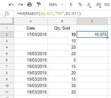
To calculate the average of non-blank cells, use the <> operator (logical NOT):

=AVERAGEIF(A2:A11, "<>", B2:B11)

4. Using Wildcards with AVERAGEIF Function

Wildcard characters (*, ?, ~) enhance flexibility with text-based conditions, and this also applies to the AVERAGEIF function:

• Asterisk (*): Matches any number of characters.
  =AVERAGEIF(B2:B6, "north*", C2:C6) This matches text like “north”, “northern”, or “northwest”.
• Question Mark (?): Matches any single character.
  =AVERAGEIF(B2:B6, "n?rth", C2:C6)
• Tilde (~): Escapes special meanings of * and ?.
  =AVERAGEIF(B2:B6, "north~*", C2:C6) Matches the literal text “north*”.

5. Case-Sensitive Matches in the AVERAGEIF Function

To perform a case-sensitive match, use the EXACT function with AVERAGEIF. Since EXACT is not an array function, wrap it with ARRAYFORMULA:

• Average for case-sensitive match of “Apple”:
  =ARRAYFORMULA(AVERAGEIF(EXACT(A2:A7, "Apple"), TRUE, B2:B7))

Here:

• EXACT(A2:A7, "Apple") returns TRUE or FALSE for each cell.
• TRUE is used as the criterion.

Resources

• How to Use REGEXMATCH in AVERAGEIF in Google Sheets
• Average of Top N Percent of the Values in Google Sheets – With or Without Conditions
• Find the Average of Visible Rows in Google Sheets