In this tutorial, we will learn how to autofill alphabetical sequences from A to Z and beyond in Google Sheets.
To autofill the alphabet in Google Sheets, there is currently no built-in feature for both capital and lowercase letters. However, effective workarounds are available!
While Google Sheets offers a built-in function for Roman numerals, it doesn’t have one specifically for sequential alphabets. But don’t worry, I’ll guide you through several workaround solutions to achieve this.
Let’s explore those formulas step by step, and feel free to choose the one that best suits your needs.
Autofill the Alphabet from A to Z in Capital Letters in Google Sheets
We will use different formulas to get the results depending on whether you want the sequence in a row or column.
Vertically (Results in a Column):
If you prefer a non-array formula, you can use the following CHAR and ROW combination.
Begin by entering the formula below into any cell: =CHAR(ROW(A1)+64)
Next, drag the formula down to generate the entire alphabet sequentially. This formula ensures accurate letter generation by starting from the first row.
If you prefer an array formula to autofill alphabetical sequences from A to Z in a single vertical column in one go, use the following CHAR and SEQUENCE combination.
=ArrayFormula(CHAR(SEQUENCE(26, 1, 65)))Both formulas would return capital letters because the ASCII character codes 65 to 90 represent uppercase letters.
Horizontally (Results in a Row):
For non-array formula lovers, I suggest the following CHAR and COLUMN combination.
Enter the following formula into any cell: =CHAR(COLUMN(A1)+64)
Drag the formula across to generate the alphabet horizontally.
Here also, we can use the array formula with just one change. You need to modify the SEQUENCE to return a sequence horizontally. Here you go.
=ArrayFormula(CHAR(SEQUENCE(1, 26, 65)))This will autofill alphabetical sequences (the letters A to Z) horizontally in the entered row.
Autofill the Alphabet from a to z in Lowercase Letters in Google Sheets
To modify the capital letter formulas for lowercase, simply replace 64 with 96 and 65 with 97. Here are the corrected formulas:
Vertically:
- Drag-down formula:
=CHAR(ROW(A1)+96) - Array formula:
=ArrayFormula(CHAR(SEQUENCE(26, 1, 97)))
Horizontally:
- Drag-across formula:
=CHAR(COLUMN(A1)+96) - Array formula:
=ArrayFormula(CHAR(SEQUENCE(1, 26, 97)))
These formulas return the alphabetical sequence of lowercase letters because the ASCII character codes 97 to 122 represent lowercase letters.
What about auto-filling alphabetical sequences beyond Z, such as AA, AB, AC, … in Google Sheets?
Autofill the Alphabet from A to Z and Beyond in Capital Letters in Google Sheets
If you need to create alphabetical sequences that extend beyond the 26-letter limit, going beyond the letter Z, you can employ a different approach. This involves using REGEXREPLACE and ADDRESS functions in conjunction with SEQUENCE, ROW, and COLUMN.
Here also, your requirements may be different. You may want the sequential alphabet vertically or horizontally. We will start with vertical sequencing of capital letters A to Z and beyond.
Vertically:
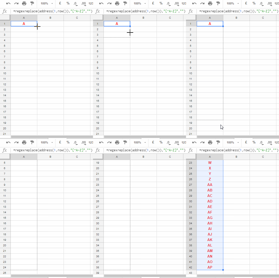
To autofill the alphabetical sequence from A to Z and beyond vertically, enter the following formula in any cell (for example, cell A1) and drag it down.
=REGEXREPLACE(ADDRESS(1, ROW(A1)), "[^A-Z]", "")
How does this formula work?
The function ADDRESS plays the main role in this formula. It returns the cell references like $A$1, $B$1, and $C$1 when dragging it down. The cell address solves the mystery of getting sequential alphabets beyond the letter Z.
Syntax: ADDRESS(row, column)
That means the formula =ADDRESS(1, 1) would return $A$1, and =ADDRESS(1, 2) would return $B$1.
From this, one thing is clear. If we can find a way to increment the column numbers (see the syntax), the ADDRESS function can return the above-said sequence (absolute cell references). We can use the ROW function for this.
=ADDRESS(1, ROW(A1))That is what I did in my formula. When you drag the formula down (I am talking about the main formula with regex), the row number gets changed. That means the row number feeds the sequential numbers 1, 2, 3, etc. to the ADDRESS.
The REGEXREPLACE function is only to remove the extra characters, the $ and row numbers, from the cell references to make it alphabets A, B, C, and so on.
Can we convert this into an array formula?
Yep! You just need to replace ROW(A1) with SEQUENCE(n) and enter it as an array formula. Here is one example.
=ArrayFormula(REGEXREPLACE(ADDRESS(1, SEQUENCE(52)), "[^A-Z]", ""))The above formula will autofill alphabetical sequences A to AZ (52 characters) vertically in Google Sheets
Horizontally:
How do we convert the above formula to autofill alphabetical sequences beyond Z horizontally in Google Sheets?
It’s quite simple. In the non-array formula, replace ROW(A1) with COLUMN(A1):
=REGEXREPLACE(ADDRESS(1, COLUMN(A1)), "[^A-Z]", "")In the array formula, make the SEQUENCE return a sequence of numbers horizontally.
=ArrayFormula(REGEXREPLACE(ADDRESS(1, SEQUENCE(1, 52)), "[^A-Z]", ""))Autofill the Alphabet from a to z and Beyond in Lowercase Letters in Google Sheets
To get lowercase letters, just wrap the above formulas with the LOWER function. In the array formula, the LOWER should be placed within the ARRAYFORMULA.
That’s all about autofilling alphabetical sequences in Google Sheets.
Resources
- Assign the Same Sequential Numbers to Duplicates in a List in Google Sheets
- Auto-Fill Sequential Dates When Value Entered in Next Column in Google Sheets
- Backward Sequence Numbering in Google Sheets
- Fill a Column with a Sequence of Decimals in Google Sheets
- How to Get Sequence of Months in Google Sheets


