A handy tip related to grouped data, that is what you are going to get from this Google Sheets tutorial on how to assign the same sequential numbers to duplicates.

If an item, for example, “Cherry”, is in row 3 in your list, the sequential number of it will be 3.

Assume, again the item is repeated in rows 4 and 5. How to get the same sequential number 3 to these duplicates using an array formula in Google Sheets?

In other words, this tutorial describes how to use an array formula to assign sequential numbers to unique values in Google Sheets.

As additional info, without any modification, my formula will work in sorted as well as an unsorted list in Google Sheets.

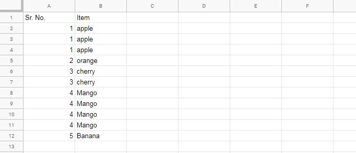
Here in this example (please refer to screenshot # 1), I have assigned the same sequential numbers (in A2:A) to duplicates in column B.

Screenshot # 1:

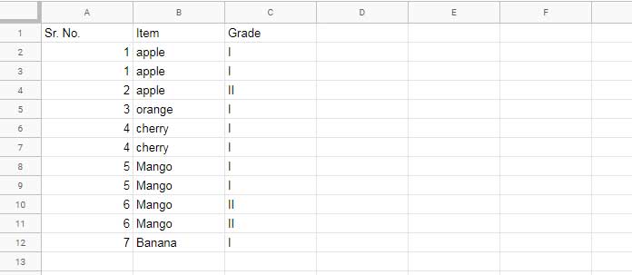
Also, in this tutorial, I’ll explain how to assign the same sequential numbers to duplicates based on 2 or more columns (please refer to screenshot # 2).

Screenshot # 2:

Array Formula to Assign the Same Sequential Numbers to Duplicates

I know some of you, probably those who are migrated from Excel or using Excel may have familiar with a non-array formula for the same.

For example, refer to my screenshot # 1. As per that list, you can type 1 in cell A2. Then in cell A3 type the following formula and drag down until reaching the cell A12.

=if(B2=B3,A2,A2+1)

This action will assign the sequential numbers to unique values and will work both in Excel and Google Sheets.

Does it justify my topic assigning the same sequential numbers to duplicates?

Nope!

Do you know why?

The result seems perfect, right? But not that much perfect. Type “apple” (without quotes) in cell B13 and copy the existing formula from cell A12 to cell A13.

It will put 6 instead of serial number 1 which is the serial number of the item “apple” in the list.

That means we can use the above non-array formula only in a sorted range to assign/generate sequential numbers to unique values in a list in Google Sheets.

The charm of my array formula (that you will get below) is that it will work in both sorted as well as un-sorted range.

Being an array formula, it will automatically expand the results up to the last row in the list even if the list is growing.

Assign Sequential Numbers to Single Column Unique Values (Screenshot # 1)

Let’s start with the array formula to assign the same sequential numbers to single column duplicates.

Just key the below formula in cell A2 and help it expand by making sure that the cells below it (cell A2) are blank.

=ArrayFormula(if(len(B2:B),match(B2:B,unique(B2:B),0),))

The formula explanation, also the logic, is always my priority. Here there is no exception.

Formula Logic and Explanation

In the formula above you can remove the if(len(B2:B), and the last comma, if you opt to use closed range B2:B12.

The above Len formula is to limit the expansion of the array formula up to the last cell containing a value.

How this array formula assigns sequential numbers to unique values in Google Sheets?

The answer lies in the question itself. It’s in the unique values.

The UNIQUE formula =unique(B2:B) returns a unique list as below.

The Match formula assigns the serial/sequential number of these items to the values in the list in B2:B.

I mean all the “apple” in the list will get the sequential number 1, “orange” will get 2 and so on.

How?

To know this you must understand how the Match works?

Syntax of the Match Function: MATCH(search_key, range, [search_type])

Purpose: Returns the relative position(s) of an item(s) in a range that matches a specified value(s).

Here the rage is =unique(B2:B) and the specified values (search_keys) to match are B2:B.

Match assigns the relative position 1 to “apple”, 2 to “orange”, 3 to “cherry”, 4 to “mango” and 5 to “banana”.

Please refer to the above table to understand the order of items (relative positions).

Assign Sequential Numbers to Multi-Column Unique Values (Screenshot # 2)

What about assigning the same sequential numbers to multi-column based duplicates in a list? Please refer to screenshot # 2 above.

Here you must evaluate duplicates from a different point of view. It’s not the mere repetition of value in one column. There are two columns involved.

If the item names (B2:B) and grades (C2:C) are the same in more than one row, then such values are duplicates.

In this case what you want to do is to add the range C2:C to B2:B within the formula.

=ArrayFormula(if(len(B2:B),match(B2:B&C2:C,unique(B2:B&C2:C),0),))

That’s all.

Conclusion

The above same technique, I mean assigning the same sequential numbers to duplicate items, I will use in advanced conditional formatting tutorial later.

The next tutorial will possibly be on that and I will leave the link below (above Additional Resources) once ready.

Additional Resources:

1. Find Missing Sequential Dates in a List in Google Sheets [Array Formula].
2. Skip Blank Rows in Sequential Numbering in Google Sheets.
3. How to Populate Sequential Dates Excluding Weekends in Google Sheets.