


")


")

")
")
 in Excel & Google Sheets")


When you have several tables within a single sheet—not across multiple sheets in a workbook—you can use 3-D references to stack the data. If the tables are arranged vertically, the stacking will occur vertically; similarly, if they are arranged horizontally, the stacking will occur horizontally.
It’s important to note that 3-D referencing is unnecessary when you only have one or two tables.
The Use of 3-D Referencing for Structured Data Tables in Sheets
Assume you have sales data for January in one table, February in another, and so on, totaling 12 tables from January to December.
You can stack these tables by using just the first and last table references. This approach simplifies data manipulation, enabling you to easily calculate total sales or category-wise totals.
When using 3-D references in structured data tables, you should pay attention to a few important factors to maintain data integrity.
Field Labels:
The stacked data will include field labels between the tables. You might want to filter these out when using functions like QUERY; otherwise, their presence may cause mixed data type issues.
For example, if your tables contain a numeric field and a label appears in that column, stacking can lead to that column having mixed data types.
To filter out these labels, ensure that you use the same field label across all tables. This way, you can match the field label and filter out all such rows.
Data Types:
Maintaining consistent data types is another critical aspect of data integrity. Each table can have a different number of columns and rows, but the data types should remain uniform. For instance, if the first column contains text and the second column contains numeric values, this pattern should be consistent across all tables. If there are discrepancies, 3-D referencing may still function, but you might encounter issues with data manipulation due to mixed data types.
Dimension:
In vertical 3-D referencing of data tables, the maximum number of columns will be determined by the larger of the first or last table.
In horizontal 3-D referencing, the number of rows is determined by the larger of the first or last table.
Vertical 3-D Referencing of Structured Data Tables
In the following example, I have three tables named Jan, Feb, and Mar, arranged one below the other.
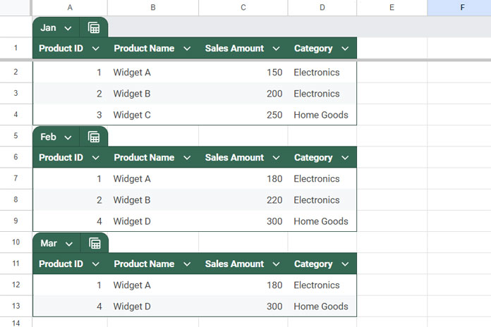
You can use the following formula to create a 3-D reference to the entire tables:
=Jan[#ALL]:Mar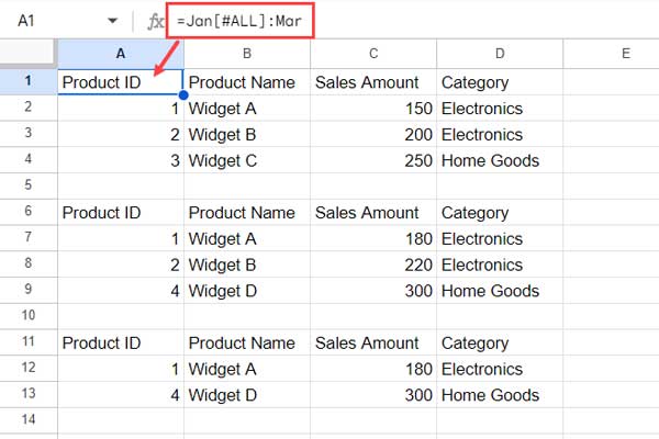
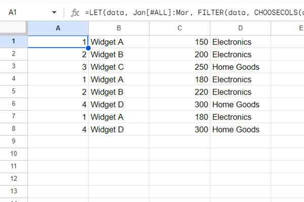
To remove the header rows (field labels) and empty rows, use the following FILTER formula:
=LET(data, Jan[#ALL]:Mar, FILTER(data, CHOOSECOLS(data, 1)<>"Product ID", CHOOSECOLS(data, 1)<>""))This formula filters out blank rows and rows containing the label “Product ID” in the first column, allowing you to manipulate the remaining data using QUERY or other functions.
What if you want to perform a vertical 3-D reference of a specific column?
To reference the ‘Sales Amount’ field in all tables, use:
=Jan[Sales Amount]:Mar[Sales Amount]You can apply the same FILTER by replacing “Product ID” with “Sales Amount” to filter out the labels:
=LET(data, Jan[Sales Amount]:Mar[Sales Amount], FILTER(data, CHOOSECOLS(data, 1)<>"Sales Amount", CHOOSECOLS(data, 1)<>""))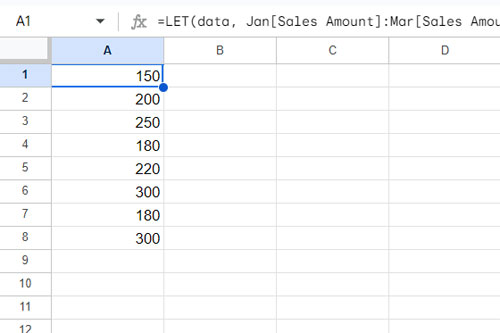
Horizontal 3-D Referencing of Structured Data Tables
Horizontal 3-D referencing is less common, but it can still be useful in certain scenarios.
Here, I have three tables named North, South, and West arranged horizontally.
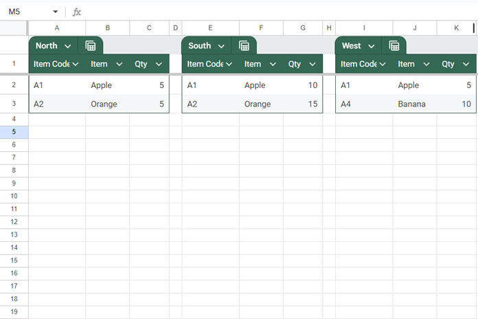
To reference them, use:
=North[#ALL]:WestIn this case, you don’t need to filter out field labels. Instead, the following formula will filter out any empty columns:
=LET(data, North[#ALL]:West, FILTER(data, CHOOSEROWS(data, 1)<>""))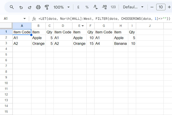
Important Note
Google Sheets does not natively support 3-D referencing for regular data. If you need this functionality, you can use my custom Named function. For more information, check out this tutorial: 3-D Reference in Google Sheets (Workaround).