The REDUCE function in Excel uses an accumulator to store intermediate values during the calculation and returns the final accumulated value.

We can use the VSTACK or HSTACK functions to vertically or horizontally stack the accumulator values at each iteration, allowing us to capture intermediate results. This combination is highly effective for solving nested array issues that may arise when using other LAMBDA functions, such as MAP.

REDUCE Function in Excel: Syntax and Formula Example

Syntax:

=REDUCE(initial_value, array, lambda(accumulator, value, calculation))

Where:

• initial_value: The starting value of the accumulator. Typically, 0 is used for numeric calculations, and "" (empty string) is used for text aggregation.
• array: The function reduces this array.
• lambda: The lambda function, which takes two arguments: the accumulator and the current value. The ‘accumulator’ stores the running total or result, starting with the initial value provided in the REDUCE function. The ‘value’ represents each element in the array.

Example of Using the REDUCE Function in Excel:

=REDUCE(0, {5, 10, 100, 200, 10, 50}, LAMBDA(a, v, a+(v>30))) // returns 3

The calculation in this formula is a + (v > 30).

If ‘v’ is greater than 30, the formula returns TRUE, which is equivalent to 1. This 1 is added to the accumulator (‘a’), and the initial value in the accumulator is 0.

The formula calculates each value in the array at every step and stores the final output in the accumulator.

Using REDUCE with VSTACK or HSTACK: A Powerful Combination

As mentioned, the REDUCE function in Excel reduces an array and returns the final output. However, you can also capture intermediate calculation values by vertically or horizontally stacking the accumulator value in each iteration.

Combining with HSTACK:

Syntax of REDUCE + HSTACK Combo:

=REDUCE(initial_value, array, lambda(accumulator, value, HSTACK(accumulator, calculation)))

Example:

In the following example, I have item names in cells A2:A9 and the corresponding category for each item in cells B2:B9.

Enter the following formula in cell D1 to get the unique categories across the row:

=TOROW(UNIQUE(B2:B9))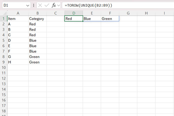

The REDUCE formula below will return the items under each category in columns:

=IFNA(DROP(REDUCE("", D1:F1, LAMBDA(a, v, HSTACK(a, FILTER(A2:A9, B2:B9=v)))), 0, 1), "")

This Excel formula essentially arranges data from rows into columns based on categories.

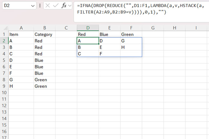
• The initial value in the accumulator is an empty string (""), and the array is the unique category in the range D1:F1.
• The calculation is HSTACK(a, FILTER(A2:A9, B2:B9=v)), where HSTACK horizontally stacks the result of the FILTER function at each intermediate step.
• The FILTER function retrieves the items associated with each category.
• The DROP function removes one column from the beginning that we don’t need, as it was added due to the initial empty string.
• IFNA replaces #N/A values with empty strings, which occurs because HSTACK pads the array to ensure equal dimensions.

Combining with VSTACK:

Syntax of REDUCE + VSTACK Combo:

=REDUCE(initial_value, array, lambda(accumulator, value, VSTACK(accumulator, calculation)))

Example:

When you arrange the source data horizontally, use the VSTACK function instead of HSTACK in the example above.

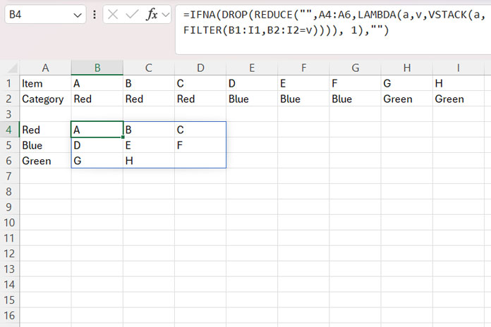
This time, the items are in B1:I1, and their corresponding categories are in B2:I2.

Enter the following formula in cell A4 to get the unique categories down the column:

=TOCOL(UNIQUE(B2:I2, TRUE))

Now, use the following REDUCE formula to arrange the corresponding items vertically:

=IFNA(DROP(REDUCE("", A4:A6, LAMBDA(a, v, VSTACK(a, FILTER(B1:I1, B2:I2=v)))), 1), "")

Here:

• The VSTACK function vertically stacks the filter outputs.
• DROP removes the first row added by the initial empty string, and IFNA replaces #N/A values with empty strings. The #N/A values are introduced by VSTACK to ensure the array dimensions are aligned correctly.

This method allows you to dynamically arrange data into rows or columns based on unique categories, providing a flexible and powerful approach to organizing data in Excel.

Examples of the REDUCE Function in Excel

Tutorials explaining advanced uses of the REDUCE function in Excel.

• Insert a Blank Row After Each Category Change in Excel
• Search Tables in Excel: Dynamic Filtering for Headers & Data
• Sum Values by Month and Category in Excel
• Combine Two Tables in Excel Using a Dynamic Array Formula