


")


")

")
")
 in Excel & Google Sheets")


Before we start applying nested column and row filtering using the FILTER function in Excel, it’s important to understand how useful it is.
When you want to dynamically filter a table by applying criteria across different columns, you can use nested column and row filters (also known as an X-Y filter).
For example, assume you have data in columns A to C, with the field labels “Item,” “Category,” and “Amount” in cells A1:C1.
You may want to filter this table by “Item” at times and by “Category” at other times, without modifying the formula.
To achieve this, enter the field label (such as “Item” or “Category”) in one cell and the corresponding criteria in another, then reference these cells in the formula.
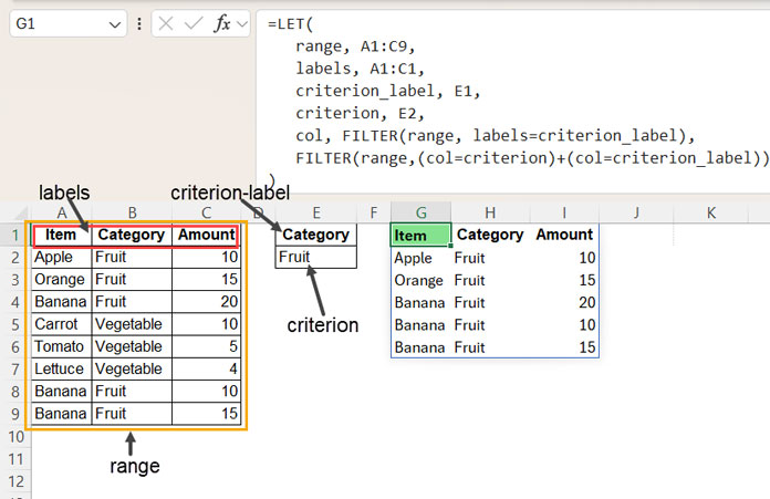
In our example, the data to filter is in A1:C9, with the criteria in E1 (the field label) and E2 (the criterion).
The formula in cell G1 will dynamically filter the data based on the criteria in E1 and E2 (the field label and the condition specified below it).
We’ll use one FILTER function nested within another, a method known as a nested filter in Excel.
How to Use Nested Column and Row Filters in Excel
Here is the simplest form of an X-Y filter formula in Excel.
=LET(
   range, A1:C9,
   labels, A1:C1,
   criterion_label, E1,
   criterion, E2,
   col, FILTER(range, labels=criterion_label),
   FILTER(range,(col=criterion)+(col=criterion_label))
)
I call it the simplest because you only need to specify the data range to filter, the first row containing the field labels, and the criteria cells (the field label for the column to filter and the condition to filter) in two separate cells.
In this formula, the arguments are as follows:
- range: A1:C9 (the range to filter)
- labels: A1:C1 (the header row reference, also called field labels)
- criterion_label: E1 (the field label of the column to filter by)
- criterion: E2 (the condition in the specified column)
To filter by the “Category” column, enter “Category” in cell E1 and one of the values from that column (e.g., “Fruit”) in E2. To filter by “Item,” enter “Item” in E1 and a corresponding value (e.g., “Apple”) in E2.
This allows you to apply nested row and column filters in Excel easily.
Formula Breakdown
In the nested column and row filters, the inner FILTER function filters columns, while the outer one filters rows.
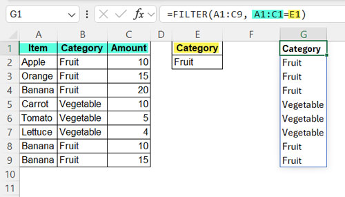
Column Filter in the Nested Filter Formula
The following formula filters the range A1:C9 based on the field label specified in cell E1:
=FILTER(A1:C9, A1:C1=E1)The result will be a single column that matches the specified label. This filtered column will then be used to further filter the range A1:C9 in the next step.
In our formula, we use the LET function to name ranges, so the above column filter becomes:
FILTER(range, labels=criterion_label)This named formula is referred to as ‘col’.
Row Filter in the Nested Filter Formula
=FILTER(A1:C9, col=E2)This formula filters the range A1:C9 based on the criterion in cell E2, using the column returned by the column filter formula.
However, the issue is that the output will lack the header row. To resolve this, we added another condition:
=FILTER(A1:C9, (col=E2)+(col=E1))The final part ensures that the output includes rows matching both the field label and the criterion in ‘col’.
The relevant part of the formula is:
FILTER(range,(col=criterion)+(col=criterion_label))This is the logic behind the nested column and row filters in Excel.