In Excel, you can use a combination of the XLOOKUP and DROP functions to extract items under a specified category from the same column.
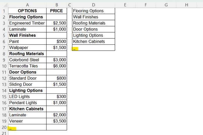
Unlike databases, Excel is flexible and allows you to enter data in various formats. Sometimes, we may have categories and their corresponding items in a single column, with prices or other details in another column. Here’s an example of such a dataset:
| OPTIONS | PRICE |
| Flooring Options | |
| Engineered Timber | $2,500 |
| Laminate | $1,000 |
| Wall Finishes | |
| Paint | $500 |
| Wallpaper | $1,500 |
| Roofing Materials | |
| Colorbond Steel | $3,000 |
| Terracotta Tiles | $6,000 |
| Door Options | |
| Standard Door | $800 |
| Sliding Door | $1,500 |
| Lighting Options | |
| LED Lights | $300 |
| Pendant Lights | $1,000 |
| Kitchen Cabinets | |
| Laminate | $2,000 |
| Veneer | $3,500 |
Objective:
Suppose you want to extract all items under the category “Kitchen Cabinets”. The items are:
- Laminate – $2,000
- Veneer – $3,500
Here’s how you can do that:
Step 1: Create a List of Categories
Let’s assume the data is in range A1:B19.
First, create a list of categories in column D. Based on the sample data, you would enter the following values in D1:D6:
- Flooring Options
- Wall Finishes
- Roofing Materials
- Door Options
- Lighting Options
- Kitchen Cabinets
Step 2: Specify the End of the List
To mark the end of the last category, enter any character below the last non-empty cell in column A (e.g., in cell A20). This character, such as an underscore (_), will act as a placeholder to signal the end of the item list for the final category. It helps to clearly define where the category items end, especially when working with flexible data in Excel.

Why is this important?
The items under each category fall between two category names. For the last category (e.g., “Kitchen Cabinets”), the boundary is unclear unless we specify this placeholder.
Similarly, enter the same character below the category list in column D—in this case, in cell D7.
Step 3: Specifying the Category and Finding the Next Category
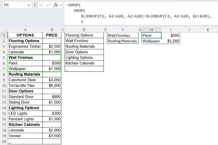
In cell F1, for example, enter the category “Wall Finishes”.
We want to extract all the items under “Wall Finishes” in the table that spans across columns A and B.
Now, in cell F2, enter the following formula:
=OFFSET(XLOOKUP(F1, D1:D6, D1:D6), 1, 0)This formula looks for the category in F1 in the list in D1:D6 and returns the corresponding value. The OFFSET function then moves one row down, pointing to the next category.
Step 4: Formula to Extract Items Under a Category from the Same Column
Now, to extract the items, use the following formula in cell H1:
=DROP(
   DROP(
      XLOOKUP(F1, A2:A20, A2:A20):XLOOKUP(F2, A2:A20, B2:B20),
      1
   ),
   -1
)
How This Formula Works:
There are two XLOOKUP functions and two DROP functions at play here:
XLOOKUP(F1, A2:A20, A2:A20): This looks for the category inF1(e.g., “Wall Finishes”) within the rangeA2:A20and returns the corresponding value from the same column (A2:A20).XLOOKUP(F2, A2:A20, B2:B20): This looks for the next category inF2within the same column range (A2:A20) and returns the corresponding value from columnB2:B20.
The colon (:) between the two XLOOKUP functions creates a range that includes all the values between the first and second XLOOKUP results.
DROP(..., 1): Removes the first row in the range (which corresponds to the category name inF1).DROP(DROP(..., 1), -1): Removes the last row in the range (which corresponds to the next category’s name).
Notes:
- This method extracts items under a specified category in the same column. The example above uses two columns (A and B). If your data spans more columns (e.g., columns
A:D), adjust the second XLOOKUP function’s range accordingly. For example, changeB2:B20toD2:D20.
Related Resources:
- XLOOKUP for First and Last Non-Blank Value in a Row
- Slicing Data with XLOOKUP in Google Sheets
- XLOOKUP in Excel: Working with Visible Rows in a Table
- Counting XLOOKUP Results with COUNTIFS in Excel and Google Sheets
- SUMIFS with XLOOKUP in Excel and Google Sheets
- Excel OFFSET-XLOOKUP: Better Alternative to OFFSET-MATCH


