We can expand an array by adding values at the end using the EXPAND function in Excel. This method is the most common way to expand an array.
However, if you want to expand the array by adding your choice of value at the beginning, you may need to use VSTACK or HSTACK in Excel.
Let’s begin with expanding an array by adding values at the end of the array using the EXPAND function in Excel.
EXPAND Function in Excel: Syntax and Arguments
Syntax:
=EXPAND(array, rows, [columns], [pad_with])Arguments:
array: The one or two-dimensional array to expand.rows: The number of rows in the expanded array. This can be omitted or greater than the number of rows in the array.columns: The number of columns in the expanded array. This can be omitted or greater than the number of columns in the array.
The formula will return a #VALUE error when the number of rows or columns specified is less than the number of rows or columns in the array.
pad_with: The value with which to pad. The default is #N/A.
Now, let’s explore how to expand an array using the EXPAND function in Excel.
Using the EXPAND Function to Expand an Array in Excel
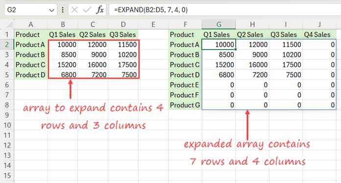
The following sales report in cell range A1:D5 shows sales figures for 4 products in Q1, Q2, and Q3.

Q4 figures are yet to come, and we have also introduced new products for which the sales figures are pending.
We want to submit a report by adding three new products at the bottom and including Q4 figures at the right-hand side of the array.
Here is how to expand the array using the EXPAND function in Excel.
Formula:
=EXPAND(B2:D5, 7, 4, 0)Where:
array: B2:D5 (the 4 * 3 array to expand)rows: 7 (the number of rows in the new array)columns: 3 (the number of columns in the new array)pad_with: 0
What about expanding the rows only?
=EXPAND(B2:D5, 7, , 0)The above formula will expand the rows only. If you want to expand the columns only, specify it as follows:
=EXPAND(B2:D5, , 4, 0)Feel free to replace 0 with "", "-", or any value you prefer for pad_with.
Using VSTACK and HSTACK Functions to Expand an Array in Excel
The EXPAND function can only expand an array by adding rows or columns at the end of the array.
If you want to expand an array by adding rows or columns at the beginning, you may need to rely on Excel’s VSTACK and HSTACK functions.
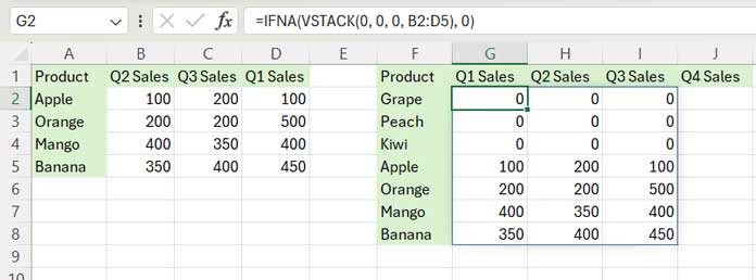
In the following example, let’s expand the data in the range B2:D5 by adding three rows at the top and one column at the left.
We will do it step by step.
Adding Rows at the Beginning of an Array:
Syntax of the Excel VSTACK Function: =VSTACK(array1, [array2],...)
If you want to add 3 rows, you should stack three 0s (array1, array2, and array3) with the range B2:D5 (array4), like this: VSTACK(0, 0, 0, B2:D5). Then wrap the formula with IFNA to replace any #N/A errors with the pad_with value 0.
=IFNA(VSTACK(0, 0, 0, B2:D5), 0)
Adding Columns at the Beginning of an Array:
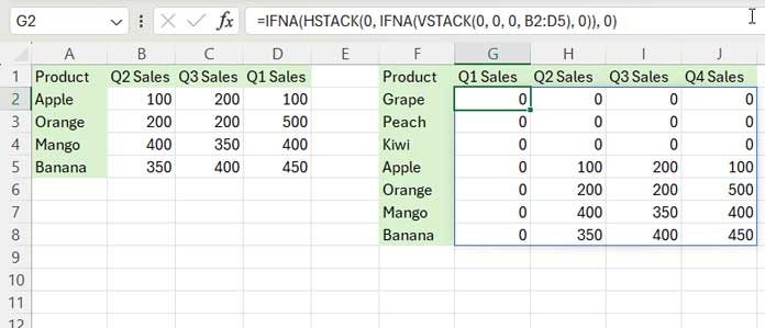
Now, we need to add columns at the beginning of this new array. For that, we can use the HSTACK function.
Syntax of the Excel HSTACK Function: =HSTACK(array1, [array2],...)
We want to add one column, so stack one 0 (array1) to the array2, i.e., IFNA(VSTACK(0, 0, 0, B2:D5), 0).
So the formula will be HSTACK(0, IFNA(VSTACK(0, 0, 0, B2:D5), 0)).
Wrap this with IFNA to replace any #N/A errors with 0 (the pad_with value).
=IFNA(HSTACK(0, IFNA(VSTACK(0, 0, 0, B2:D5), 0)), 0)
Note: When you want to pad with a hyphen, replace 0 with "-". Non-numeric characters must be entered with double quotes.
Resources
Here are some other Excel tips and tricks that are rare to find and truly unique.


