


")


")

")
")
 in Excel & Google Sheets")


In this tutorial, we will explore the purpose of OFFSET-MATCH in Excel and how OFFSET-XLOOKUP becomes a better alternative.
We use Excel’s OFFSET and MATCH combination to offset from a starting cell to a certain number of rows or columns based on the MATCH result. From that point, you can offset left, right, up, or down and return a single value or multiple values by specifying width and height.
The OFFSET and XLOOKUP combination can return similar results in Excel. However, the key difference is that the ‘reference,’ which is the OFFSET starting cell, is dynamic. The ‘reference’ is the XLOOKUP result itself.
The ‘reference’ is the key difference between OFFSET-MATCH and OFFSET-XLOOKUP in Excel. It’s a static cell reference in the former, whereas in the latter, it’s the lookup value.
In addition, XLOOKUP is a modern lookup function, and you can take advantage of its additional benefits. You can look up values from top to bottom, bottom to top, left to right, and right to left.
As a side note, VLOOKUP won’t work similarly with OFFSET. It seems to me that this is why the OFFSET and XLOOKUP combination is not yet familiar among Excel users. They might think that this combination won’t work.
Sample Data:
| Quarter | Month | Ben | Lisa |
| Q1 | January | 5000 | 4500 |
| February | 5200 | 4600 | |
| March | 5300 | 4700 | |
| Q2 | April | 5400 | 4800 |
| May | 5500 | 4900 | |
| June | 5600 | 5000 | |
| Q3 | July | 5700 | 5100 |
| August | 5800 | 5200 | |
| September | 5900 | 5300 | |
| Q4 | October | 6000 | 5400 |
| November | 6100 | 5500 | |
| December | 6200 | 5600 |
Examples of the OFFSET and MATCH Combination in Excel
The above sample data in A1:D13 is a sales summary of two employees for one year. Let’s apply the OFFSET-MATCH combination to this data.
Example 1:
Let’s first extract the sales amount of Ben in October.
=OFFSET(B1, MATCH("October", B1:B13, 0)-1, 1)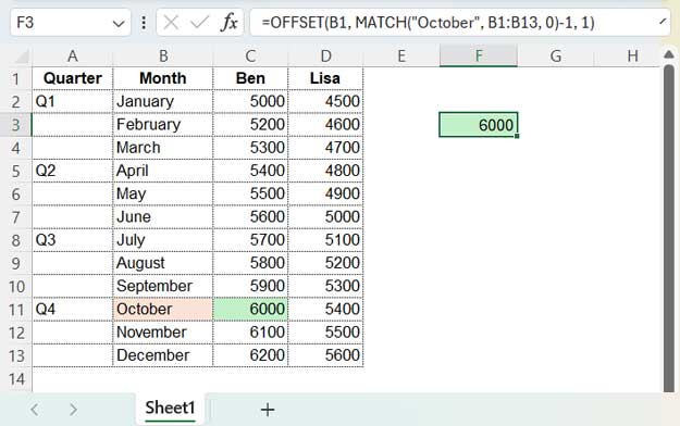
The MATCH function here matches the key “October” in B1:B13 and returns the relative position of the keyword.
MATCH Syntax:
MATCH(lookup_value, lookup_array, [match_type])Where lookup_value is “October”, lookup_array is B1:B13, and match_type is 0, which means an exact match of the lookup_value.
It would return 11. Now take a look at the OFFSET syntax:
OFFSET Syntax:
OFFSET(reference, rows, cols, [height], [width])The reference here is cell B1 from which to start the offset of rows and columns.
rowsis the MATCH result – 1 because the offset count starts from 0.colsis 1 since we want the result from column C.
Example 2:
Actually, we don’t require the above type of lookup since we can use VLOOKUP for that.
=VLOOKUP("October", B1:C13, 2, 0)But here is why the combination is a powerful alternative to VLOOKUP.
=OFFSET(A1, MATCH("Q4", A1:A13, 0)-1, 1, 3, 2)This formula will return the Q4 sales of Ben.
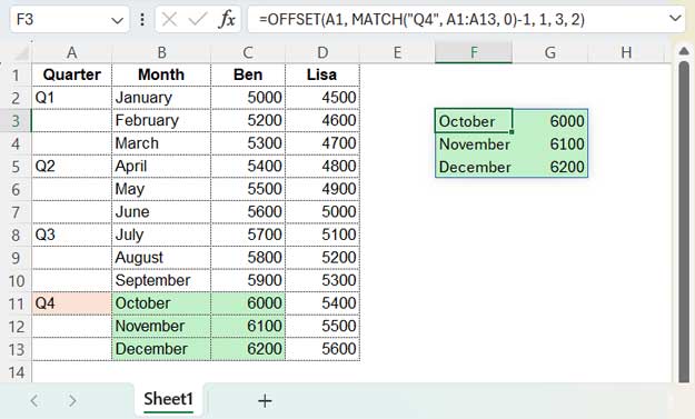
The OFFSET returns the relative position of “Q4” in column A. The OFFSET offsets match-1 row and 1 column and returns 3 rows (height) and two columns (width).
This wouldn’t be doable with VLOOKUP in a regular way.
Note:
The above examples are for vertical lookups. If you perform a horizontal lookup, the MATCH formula should be used in the ‘cols’ argument of the OFFSET function.
Examples of the OFFSET and XLOOKUP Combination in Excel
The drawback of the above OFFSET and MATCH combination in Excel is that it offsets from a specified starting cell. If you want to go beyond static lookups, try the OFFSET and XLOOKUP combination.
First of all, XLOOKUP is currently not available in all versions of Excel. Please check the availability before testing. If you are using Excel 2019 or any earlier version, the following formulas won’t work.
To look up a value and offset around it, you can use this OFFSET-XLOOKUP combination formula:
=OFFSET(XLOOKUP("October", B2:B13, B2:B13), 0, 1)The XLOOKUP function searches for “October” in the range B2:B13 and returns the value “October” from the same range.
XLOOKUP Syntax:
=XLOOKUP(lookup_value, lookup_array, return_array, [if_not_found], [match_mode], [search_mode]) Where lookup_value is “October”, lookup_array and return_array are B2:B13.
We can use the XLOOKUP result as the reference in OFFSET. In the above example, the OFFSET function offsets 0 rows and 1 column from the XLOOKUP result and returns Ben’s October sales.
The following formula searches for the key “Q4” and returns Ben’s sales in October, November, and December.
=OFFSET(XLOOKUP("Q4", A2:A13, A2:A13), 0, 1, 3, 2)The XLOOKUP function searches for “Q4” in A2:A13 and returns “Q4”. The OFFSET function offsets 0 rows and 1 column. The height of rows is 3 and the width of columns is 2.
Wrap-up
In the OFFSET and MATCH combination, the reference to offset is a static cell reference. MATCH is used either to offset rows (in vertical lookups) or columns (in horizontal lookups), so it is not dynamic.
In the OFFSET and XLOOKUP combination, the reference to offset is the XLOOKUP result itself, making it more dynamic.
You will find these two combinations useful in scenarios where you need to return values from around the lookup value.
They are also helpful in handling merged cells in lookups. Regular lookup functions may match the value in the very first cell of the merged cells. You can look up that value and offset to get the values corresponding to the merged cell.