
")

")
")


")


")


You might know how to use the FILTER function to filter data based on a criterion selected from a dropdown list in Excel. But what if you want to include an ‘All’ option in the dropdown to display all data?
In this tutorial, I’ll explain how to filter data using a dropdown selection, and also how to display the entire dataset when the dropdown value is set to “All.”
For example, consider the sample data in columns A to C, with the dropdown in cell E2.
The formula in G2 filters the data based on the value selected in E2. If the value in E2 is “All,” the formula returns the entire dataset.
Now, let’s walk through the step-by-step instructions.
Creating a Unique List with an “All” Option
Our sample data is in the range A1:C100, with headers in the first row.
We’ll filter the data based on the values in column A. The first step is to create a unique list from these values and add the “All” option at the top.
Enter the following formula in cell L2:
=VSTACK("All",TOCOL(UNIQUE(A2:A100),1))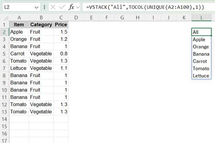
- The UNIQUE function returns the distinct values from the range A2:A100, excluding A1, which contains the header.
- Any blank cells in column A will cause an empty row at the end of this unique list. The TOCOL function removes this empty cell.
- The VSTACK function then stacks the “All” option at the top of the unique list.
We’ll use this list to create a dropdown, which will be used to filter the data.
Setting Up a Drop-Down List
- Navigate to cell E2.
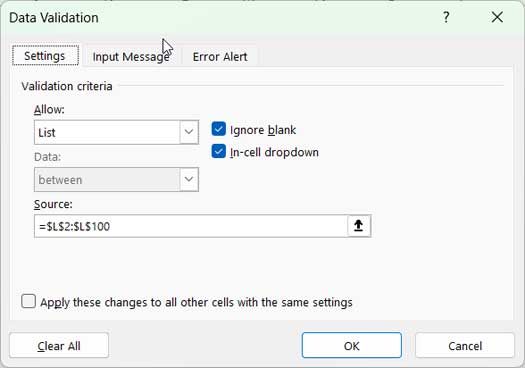
- Go to the Data tab and, under Data Tools, click Data Validation.
- In the Allow field, select List from the dropdown.
- In the Source field, enter
=$L$2:$L$100, which represents the range of unique values. - Click OK.
Now, you’re ready to filter the data using the values from the dropdown list in cell E2. When you open the dropdown, you’ll see that the list includes the “All” option.
Formula to Filter Data Based on the Dropdown Selection
To start, let’s create a formula that filters the data based on the selected dropdown value, excluding the “All” option.
Enter the following formula in cell G2:
=FILTER(A2:C100, (A2:A100=E2)*(A2:A100<>""),"Please select a value from the dropdown")This formula filters the data in columns A to C according to the value selected in cell E2. If E2 is empty or set to “All,” the formula will return “Please select a value from the dropdown.”
The formula follows this syntax:
FILTER(array, include, if_empty)- array:
A2:C100(the range to filter) - include:
(A2:A100=E2)*(A2:A100<>""), which means the values in column A must match the dropdown selection in E2 and not be blank.
When there are no matching results, the formula outputs “Please select a value from the dropdown,” which is specified in the if_empty argument.
Filtering Data with a Dropdown and “All” Option – Formula Adjustments
To include the “All” selection option in the FILTER formula, you need to adjust the include argument to handle this option.
Replace (A2:A100=E2) with IFNA(XMATCH(A2:A100, IF(E2="All", A2:A100, E2)), 0).
The final formula to filter data based on the drop-down selection, including the “All” option, will be as follows:
=FILTER(A2:C100, IFNA(XMATCH(A2:A100, IF(E2="All", A2:A100, E2)), 0)*(A2:A100<>""), "Please select a value from the dropdown")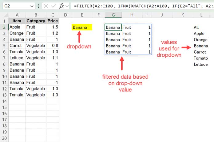
What does the new include part, i.e., IFNA(XMATCH(A2:A100, IF(E2="All", A2:A100, E2)), 0), do in the formula?
This part uses the XMATCH function with the following syntax:
XMATCH(lookup_value, lookup_array)Where:
- lookup_value:
A2:A100 - lookup_array:
IF(E2="All", A2:A100, E2).
The lookup_array returns the values in A2:A100 if E2 is “All”; otherwise, it returns the value in E2.
XMATCH searches for the lookup_value in the lookup_array and returns the relative position of the matching value(s) within the lookup_array. If no match is found, it returns #N/A errors. The IFNA function converts these #N/A errors to 0.
Here is what the above part returns when the lookup_array is E2.
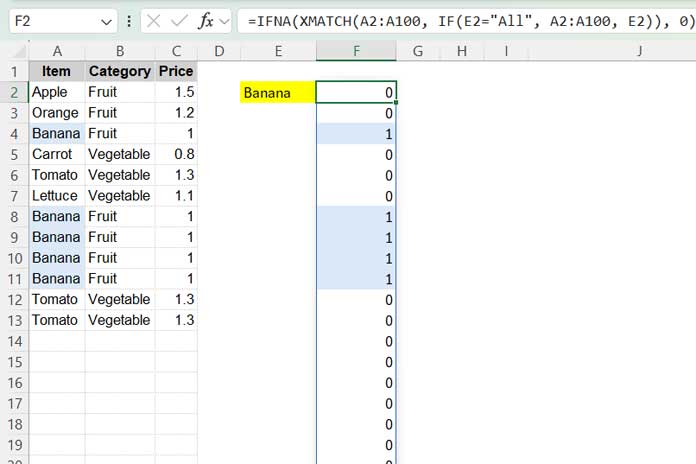
The FILTER function then filters the data wherever XMATCH returns a value greater than 0, indicating a match.