This tutorial introduces a unique formula to add a dynamic total row to your Excel FILTER function results.

Key Features of the Formula

• Easy to Use: Simply input your FILTER formula and specify the column numbers for the sum. The formula automatically places the total.
• Flexible Column Totals: You can easily add totals to multiple columns, or to all columns except the first, as you reserve it for the label “Total.”
• Adaptable to Any FILTER Formula: The formula works regardless of the number of columns or rows in the FILTER function results.
• Compatible with Google Sheets: You can use this formula in Google Sheets with just one minor adjustment.

We will first look at the formula, followed by examples of how to use it with different FILTER formulas in Excel. Afterward, we’ll dive into a detailed explanation of the formula for those interested.

Dynamic Total Row Formula for Excel FILTER Function

Generic Formula:

=LET(data, filter_formula, cols, HSTACK(2, 3, 4, ...), total, BYCOL(data, LAMBDA(val, SUM(val))), fnl, IF(XMATCH(SEQUENCE(1, COLUMNS(total)), cols), total), final, IFNA(HSTACK("Total", CHOOSECOLS(fnl, SEQUENCE(COLUMNS(fnl)-1, 1, 2))), ""), VSTACK(data, final))

In this formula, you need to make two changes:

1. Replace filter_formula with your actual FILTER function.
2. Specify the column numbers in HSTACK(2, 3, 4, …) to determine the columns under which to place the total. For example, if you specify 2, 5, the total will be placed under the second and fifth columns. Do not specify 1, as the first column is reserved for the “Total” label.

When you copy and paste the generic formula, remove the “=” sign first. After replacing the placeholder text and column numbers, add the “=” sign back. Alternatively, you can place an apostrophe in front of the equal sign, like '= to turn it into text. Once you’ve replaced the placeholder text with your FILTER formula, you can remove the apostrophe.

This is the easiest way to add a total row to your FILTER function results in Excel.

Example: Adding a Dynamic Total Row to Excel FILTER Function Results

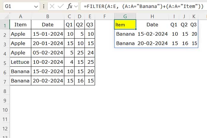
In the following example in an Excel spreadsheet, I have item names in column A, the date of receipt in column B, and quantities received in Q1, Q2, and Q3 in columns C to E.

The following formula will filter the rows where the values in the first column match either “Banana” or “Item”:

=FILTER(A:E, (A:A="Banana")+(A:A="Item"))

The +(A:A="Item") part ensures that the formula returns the header row.

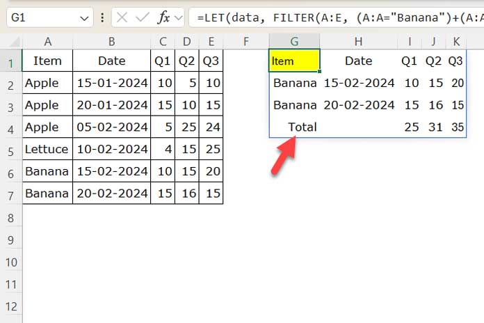
I want to add a total row at the bottom of the formula result to sum the quantities in the 3rd, 4th, and 5th columns.

In our generic formula, replace the placeholder text filter_formula with the above FILTER formula and HSTACK(1, 2, 3, …) with HSTACK(3, 4, 5).

Formula:

=LET(data, FILTER(A:E, (A:A="Banana")+(A:A="Item")), cols, HSTACK(3, 4, 5), total, BYCOL(data, LAMBDA(val, SUM(val))), fnl, IF(XMATCH(SEQUENCE(1, COLUMNS(total)), cols), total), final, IFNA(HSTACK("Total", CHOOSECOLS(fnl, SEQUENCE(COLUMNS(fnl)-1, 1, 2))), ""), VSTACK(data, final))

This will add a dynamic total row to the bottom of the FILTER function results.

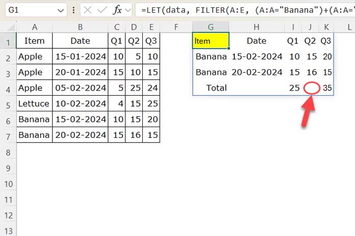
When you replace HSTACK(3, 4, 5) with HSTACK(3, 5), you will get the following output.

Formula Breakdown

This section is for those who want to understand the logic behind the formula. Feel free to skip this part if you're not interested in the details.

We use the LET function to assign names to formula expressions and reuse those names in the calculations.

• data: FILTER(A:E, (A:A="Banana")+(A:A="Item"))
  Refers to the filter formula.
• cols: HSTACK(3, 4, 5)
  Refers to the columns for which totals need to be calculated.
• total: BYCOL(data, LAMBDA(val, SUM(val)))
  The BYCOL function processes each column in the ‘data’ array and sums it up. It calculates totals for all columns in the FILTER result, regardless of whether they contain text, dates, or numbers.
• fnl: IF(XMATCH(SEQUENCE(1, COLUMNS(total)), cols), total)
  This checks if the columns in ‘total’ match the specified ‘cols.’ If there’s a match, it returns the corresponding totals, ensuring totals are only added to the desired columns.
• final: IFNA(HSTACK("Total", CHOOSECOLS(fnl, SEQUENCE(COLUMNS(fnl)-1, 1, 2))), "")
  This removes the first column from ‘fnl’ and adds the label “Total” to the final output.
• VSTACK(data, final): This stacks the ‘final’ (containing the total row) below the ‘data’ (FILTER formula result).

This is how we dynamically add a total row below the FILTER function results in Excel.

Is the Dynamic Total Row for Excel FILTER Compatible with Google Sheets?

Yes! The above formula is fully compatible with Google Sheets. The only thing you need to do is enter it as an array formula. Simply wrap the formula with the ARRAYFORMULA function in Google Sheets.

So the generic formula will be:

=Array_Formula(LET(data, filter_formula, cols, HSTACK(1, 2, 3, ...), total, BYCOL(data, LAMBDA(val, SUM(val))), fnl, IF(XMATCH(SEQUENCE(1, COLUMNS(total)), cols), total), final, IFNA(HSTACK("Total", CHOOSECOLS(fnl, SEQUENCE(COLUMNS(fnl)-1, 1, 2))), ""), VSTACK(data, final)))

Resources

• Dynamic Total Row for FILTER, QUERY, or ARRAY Results in Sheets
• Formula to Insert Group Total Rows in Google Sheets
• Blank Cell between Two Totals in Query Total Row in Google Sheets
• Insert Subtotal Rows in a Google Sheets Query Table
• How to Add a Total Row to a Google Sheets Data Table