")
")


")


")

")
")
 in Excel & Google Sheets")


This tutorial explains how to create a dynamic moving average in Excel that spills the average down the column and adjusts based on the window size.
A moving average, also referred to as a rolling or running average, involves analyzing data points by calculating a series of averages from various subsets within the entire data set.
In Excel 365 or versions that support dynamic arrays, you can automate this process using advanced functions.
How it works:
- You specify a window size in the formula that determines the number of data points included in each average.
- The formula calculates the average for the first set of data points and returns it in the last row of the first window. Then, it returns the average of the next subset in the next row and continues until the last row of the data set.
Essentially, you can use it to return a 2-day, 3-day, or n-day moving average in Excel, where n represents the window size. That’s why we call it a dynamic moving average.
Example:
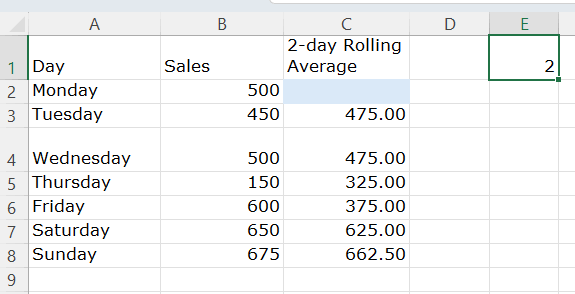
In the following example, the second column contains the sales data for one week, and the third column shows the 3-day rolling average.
| Day | Sales | 3-day Rolling Average |
| Monday | 500 | |
| Tuesday | 450 | |
| Wednesday | 500 | 483.33 |
| Thursday | 150 | 366.67 |
| Friday | 600 | 416.67 |
| Saturday | 650 | 466.67 |
| Sunday | 675 | 641.67 |
Let’s automate this calculation using a dynamic moving average formula in Excel.
Step 1: Formatting the Data
We need sample data to test. So, either copy and paste the above data (only the first and second columns) into cells A1:B8 in your Excel spreadsheet or enter the above data manually.
Step 2: Specifying the Window Size
Assume you want a 3-day moving average. Enter 3 in cell E1 so that you can easily switch the window size later by simply editing this number. Yes! The moving average should be dynamic in all aspects.
Step 3: Formula for Dynamic Moving Average in Excel
Enter the following formula in cell C2 to get the rolling average. Don’t forget to enter the field label “Rolling Average” in cell C1.
=LET(data,B2:B8,window,E1,seq,SEQUENCE(ROWS(data)),TAKE(IFERROR(VSTACK(DROP(EXPAND("",window),1),MAP(seq,LAMBDA(seqA,AVERAGE(FILTER(data,(seq>=seqA)*(seq<seqA+window)))))),""),MAX(seq)))When using this formula, replace:
B2:B8with your data range.E1with the cell reference containing the window size. Enter 2 for a rolling 2-day average, 3 for a rolling 3-day average, and so on, in that cell.
Note: Optionally, in cell C1, you can enter =E1 & "-day Rolling Average" to get the dynamic field label based on the window size specified in cell E1.
Dynamic Moving Average: Formula Breakdown
I understand the importance of a formula breakdown as it can help Excel users who wish to improve their skills with advanced formulas.
Here is a step-by-step explanation of how to code the dynamic moving average formula in Excel so that you can understand it better.
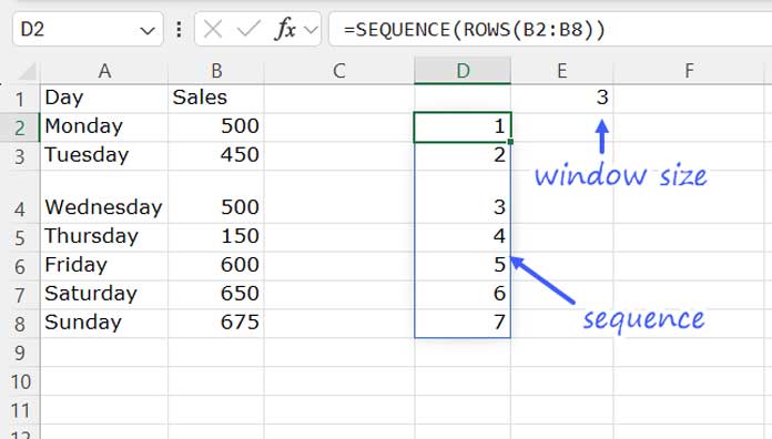
- Generate Sequence Numbers
First, generate sequence numbers that match the total data points. Use the following formula in cell D2:
=SEQUENCE(ROWS(B2:B8))- Specify the Window Size
Enter the window size in cell E1 (for example, 3).
- Calculate the Average for the First Window
Use the following formula in cell C2 to calculate the average of the data points in the first window size:
=AVERAGE(FILTER($B$2:$B$8, ($D$2:$D$8 >= D2) * ($D$2:$D$8 < D2 + $E$1)))The FILTER function extracts data points where the sequence number is between 1 and the window size.
- Make It Dynamic
To make the formula dynamic and ensure it spills down correctly, use the MAP function. This function iterates over the sequence array:
=MAP(D2:D8, LAMBDA(seqA, AVERAGE(FILTER(B2:B8, (D2:D8 >= seqA) * (D2:D8 <seqA + E1)))))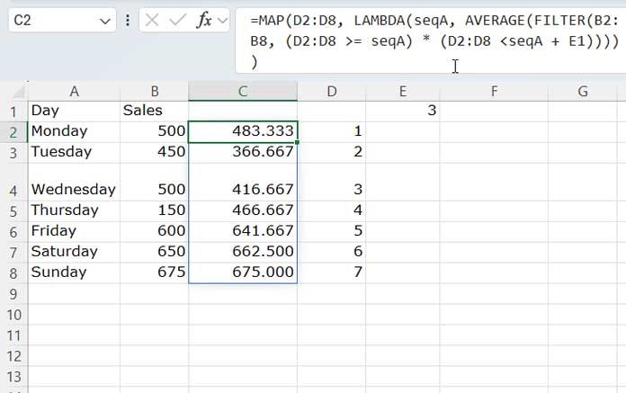
- Offset Rows at the Top Based on the Window Size
Use DROP(EXPAND("", E1), 1) to adjust the rows at the top of the moving average. EXPAND creates an array of empty string + #N/A errors based on the window size, and DROP removes the first value. See how to apply this in the next step below.
- Combine with MAP and Handle Errors
Append the MAP function result with the DROP function and wrap it with IFERROR to remove errors:
=IFERROR(VSTACK(DROP(EXPAND("", E1), 1), MAP(D2:D8, LAMBDA(seqA, AVERAGE(FILTER(B2:B8, (D2:D8 >= seqA) * (D2:D8 <= seqA + E1 - 1)))))), "")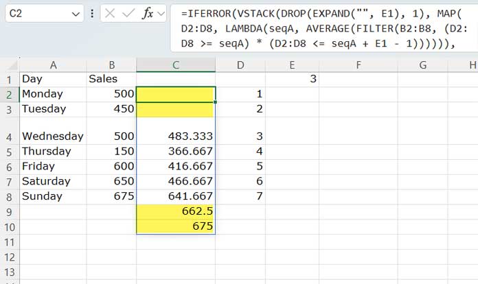
- Limit the Number of Rows
Finally, limit the number of rows in the result to match the total number of data points using the TAKE function:
=TAKE(IFERROR(VSTACK(DROP(EXPAND("", E1), 1), MAP(D2:D8, LAMBDA(seqA, AVERAGE(FILTER(B2:B8, (D2:D8 >= seqA) * (D2:D8 <= seqA + E1 - 1))))), ""), ROWS(B2:B8))This formula provides a dynamic array formula to calculate the moving average in Excel.
You can replace D2:D8 with the SEQUENCE formula from cell D2 to remove the helper sequence range. Additionally, use LET to name value expressions and simplify the formula. You can see the cleaned-up version in my original formula.