Would you like to create a sequence of dates in every nth row in Excel using a dynamic array formula? This tutorial will guide you through the process.

When Is This Useful?

Imagine you have seven employees who work every day, and you want to insert a date sequence in column A, populating every seventh row with a date while leaving blank rows in between. This setup allows you to record daily attendance, start and end times, and other details for each employee in the adjacent columns.

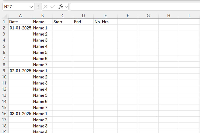
In this tutorial, we’ll cover how to create a date sequence that appears at every nth row in Excel and include a bonus formula to automatically fill employee names alongside each date.

How to Create a Sequence of Dates at Every Nth Row in Excel

To create a sequence of dates that appears at every 7th row in column A, starting from row 2, use the following formula in cell A2:

=LET(
   dt, SEQUENCE(ROWS(A1:A2555), 1, "2025-1-1", 1/7), 
   IF(MOD(ROW(A1:A2555), 7)=1, CEILING(dt, 1),"")
)

Apply Date Formatting: After entering the formula, select column A, go to the Home tab, and select Short Date under the Number group. This will format the results as dates.

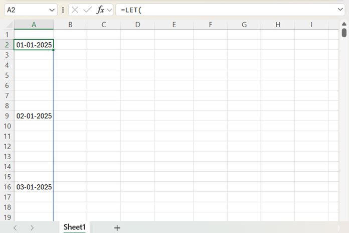
This formula generates a year-long calendar starting from January 1, 2025, with each date appearing at every 7th row. The reference A1:A2555 is used because 2555 is a multiple of 365 days and 7 rows, covering all rows for one year.

Can I use this formula starting in any row without modifying ranges?

Yes, you can!

Customizing the Date Sequence Interval Between Dates

If you want a different interval, such as a date every 5 rows, adjust the formula as follows:

1. Replace 1/7 with 1/5 to specify the increment.
2. Update MOD(ROW(A1:A2555), 7) to MOD(ROW(A1:A1825), 5) for the 5-row interval. Here, 1825 represents the total number of rows needed for a full year’s worth of dates, with each date appearing every 5th row (5 * 365 = 1825)

The revised formula for a 5-row interval would look like this:

=LET(
   dt, SEQUENCE(ROWS(A1:A1825), 1, "2025-1-1", 1/5), 
   IF(MOD(ROW(A1:A1825), 5)=1, CEILING(dt, 1),"")
)

Formula Breakdown

1. SEQUENCE(ROWS(A1:A2555), 1, "2025-01-01", 1/7): Creates a sequence of dates (date values) starting from “2025-01-01”, incrementing by 1/7 for each cell in the range. This sequence is named dt in the formula using LET.
2. IF(MOD(ROW(A1:A2555), 7)=1, CEILING(dt, 1), ""): This part of the formula returns the date in every 7th row and leaves the other rows blank.
   • MOD(ROW(A1:A2555), 7)=1: Returns TRUE only at every 7th row, allowing the date to appear there.
   • CEILING(dt, 1): Rounds up the date to ensure it displays as a full date.

The IF function keeps dates in every 7th row, leaving other cells as blank text (“”).

Additional Tip: Automatically Fill Employee Names in Column B

If you’d like to fill in employee names next to each date in column B, enter the following formula in cell B2:

=LET(
   week, IF(LEN(A2#), {"Name 1", "Name 2", "Name 3", "Name 4", "Name 5", "Name 6", "Name 7"},""), 
   ftr, FILTER(week,CHOOSECOLS(week,1)<>""), 
   TOCOL(ftr)
)

This will fill B2:B8 with 7 employee names for the date in A2, B9:B15 for the next date, and so on.

How Does This Formula Work?

• IF(LEN(A2#), {"Name 1", "Name 2", "Name 3", "Name 4", "Name 5", "Name 6", "Name 7"}, ""): Checks for a date in the corresponding cell in column A. If a date is found, it assigns the array of employee names next to that date; otherwise, it leaves the cell blank.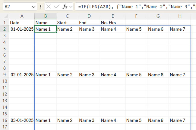
  
• FILTER(week, CHOOSECOLS(week, 1) <> ""): Filters out any empty cells, ensuring that only the names for rows with dates are included.
• TOCOL(ftr): Converts the filtered array into a column format, distributing names vertically next to each date.

This setup provides a clear and organized structure to track daily attendance, start and end times, or other details for each employee.

This tutorial shows you a dynamic way to generate a date sequence with specific row intervals in Excel. With this setup, you can automate filling employee names for each date, making it easy to track attendance and other information.

Resources

• Creating Custom Descending Sequence Lists in Excel
• Insert a Blank Row After Each Category Change in Excel
• Creating Sequential Dates in Equally Merged Cells in Google Sheets
• How to Populate Sequential Dates Excluding Weekends in Google Sheets
• Auto-Fill Sequential Dates When Value Entered in Next Column in Google Sheets
• Adding N Blank Rows to SEQUENCE Results in Google Sheets