


In this post, I’m sharing a named function to remove duplicates by a key column. The said named function supports using more than one table.
So you can combine one or more similar type tables and remove duplicates by a key column in a flash.
When I say similar type table, I mean the number of columns in both tables should match and also the data type.
The best way to remove duplicates by a key column in Google Sheets is by using the SORTN function.
I have got an example of this already here — Remove Duplicate Rows Based on Selected Columns in Google Sheets.
When there are two tables, you can append them vertically using the VSTACK function and then use that appended array within the SORTN.
But when you have several tables, you may require to specify all of them within the VSTACK. It will lengthen the formula. Also, you may require to remove blank rows in the appended array.
All this may not be easy for a novice user of Google Sheets. Here wins my named function.
The simplest way to remove duplicates by a key column is using my named function called MERGE_TABLE_REMOVE_DUPLICATES.
It can combine tables and remove duplicates by a key column in one go.
It works like this.
Assume, there are two tables in the range A2:I in Sheet tabs “Table 1” and “Table 2.”
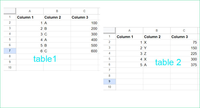
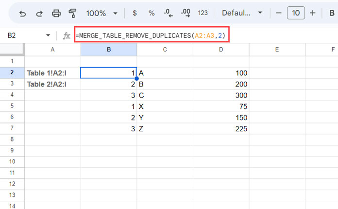
Enter Table 1!A2:I in cell A2 and Table 2!A2:I in cell A3 in a new tab and insert the following formula in cell B2 there.
=MERGE_TABLE_REMOVE_DUPLICATES(A2:A3,2)The above simple formula will combine those tables and remove duplicates by the key column # 2.
Note:- You may scroll down and copy my Sheet to see this in action.
MERGE_TABLE_REMOVE_DUPLICATES: Syntax and Arguments
The MERGE_TABLE_REMOVE_DUPLICATES is a custom-named function. So you must first import it into your Sheet before start using it.
You will get those instructions after the syntax part below.
Syntax: MERGE_TABLE_REMOVE_DUPLICATES(array_ref, key_col)
array_ref: The cell or cell range that contains the table range references.
key_col: The column that determines the duplicates. Let’s consider an employee list that contains employee names in A1:A, IDs in B1:B, and salaries in C1:C. We should specify # 1 as the key column to remove any duplicate names from this table.
The above are the syntax and arguments of the MERGE_TABLE_REMOVE_DUPLICATES named function.
In the above Google Sheets function, there are only two arguments. None of them are optional. Leaving one of them may result in the following #N/A syntax error.
Wrong number of arguments to MERGE_TABLE_REMOVE_DUPLICATES. Expected 2 arguments, but received 1 arguments.
Salient Features
- It easily removes duplicates based on a user-specified column in the range.
- The output will be a new array which will update when you edit the source range.
- If you feed multiple ranges to the MERGE_TABLE_REMOVE_DUPLICATES function, it appends them and considers them a single table before the execution.
- The result of the custom function will keep the order of the records in the source data. It won’t sort, unlike the SORTN approach mentioned at the beginning.
How To Remove Duplicates by Key Column in Google Sheets
Here are a few formula examples to help you understand how to use MERGE_TABLE_REMOVE_DUPLICATES named function.
Before that, you must import my named function into your Sheet. You can do that very quickly. Here is how.
- First, get a copy of my above Sheet.
- Open your Sheet in which you want to use my function and go to Data > Named function > Import function.
- Locate the Sheet that you just copied and select Insert.
- Select the function and Import.
Here are the steps to remove duplicates in the range C50:D100 in the “January” tab based on the key column range D50:D100.
- Enter January!C50:D100 in cell A1 in another Sheet.
- Enter 2 (key column number) in cell A2 in that Sheet.
- Time to copy-paste the following MERGE_TABLE_REMOVE_DUPLICATES formula in cell B1.
=MERGE_TABLE_REMOVE_DUPLICATES(A1, A2)Combine Tables and Remove Duplicates
Assume we have January, February, March, and April data in ranges January!C50:D100, February!C50:D100, March!C50:D100, and April!C50:D100.
Here are the steps to combine these tables and remove duplicate rows by key column # 2.
- Enter January!C50:D100, February!C50:D100, March!C50:D100, and April!C50:D100 in cell A1, A2, A3, and A4 in another Sheet.
- Enter 2 (key column number) in cell A5 in that Sheet.
- Copy-paste the following formula into cell B1.
=MERGE_TABLE_REMOVE_DUPLICATES(A1:A4, A5)That’s all. Merging tables and removing duplicates based on a specific column can’t be much easier than this.