


Usually, when you drag a formula across, you won’t get the reference down in Google Sheets.
If you think making the row relative and column absolute would serve the purpose, it won’t.
It will work when copy-pasting the formula down.
Here are three formula options from which you can choose the best one for the said purpose.
They are Index, Offset, and Indirect based.
Choose the one that you feel is easy to learn.
In the end part, we can see a real-life example of the purpose of dragging a formula across and getting the row reference down.
As a side note, we have discussed achieving the opposite of the above in another tutorial here – Change Column Letter When Formula Copied Down in Single Column.
Drag a Formula across But Get the Reference from Down – Formula Options
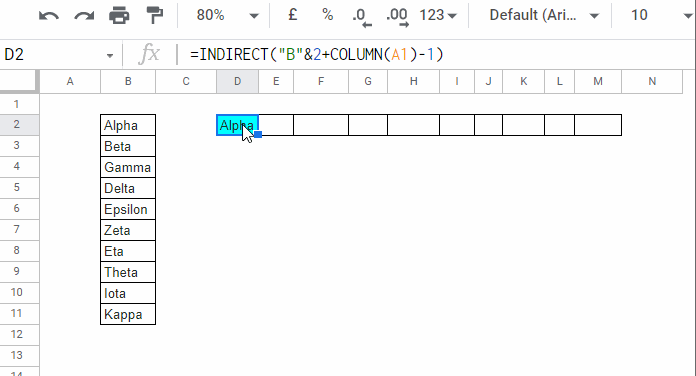
I have a list that contains text strings in cell range B2:B11 that are the first ten Greek Alphabet names.
Let’s see what happens when we use a regular formula in cell D2 and drag it across.
=$B2It will return “Alpha” in D2, E2, F2, and so on as the alphabet’s name in B2 is “Alpha.”
In the formula above, the column reference is absolute, and the row reference is relative.
When you drag/copy the above formula across, it won’t relatively change the reference down.
Here are three formulas that you can use here. The first one is based on an INDIRECT and COLUMN combination.
1. INDIRECT and COLUMN Based:
=INDIRECT("B"&2+COLUMN(A1)-1)You may insert this formula in cell D2 and drag/copy-paste it across/horizontally.
Here are the other two alternative formulas that use INDEX or OFFSET as a replacement for INDIRECT.
2. INDEX and COLUMN Based:
=index($B$2:$B$11,column(A1))3. OFFSET and COLUMN Based:
=offset($B$2:$B$11,column(A1)-1,0,1)The above formulas copy the Greek Alphabet names in a vertical list to a horizontal list.
When you drag the above formulas across, it will take the row reference from down.
The real purpose of using one of the above formulas is not simply to change the orientation of the data.
If that’s the sole purpose, then we have a better alternative in TRANSPOSE.
Empty D2:M2 and insert the following TRANSPOSE in cell D2.
=TRANSPOSE(B2:B11)The only drawback of this method is, if you don’t want any particular value in any cell in the output range, you can’t delete that.
Real Life Use
Drag a formula across but get the cell reference from down – What’s the real-life use of it?
Here is an example of this.
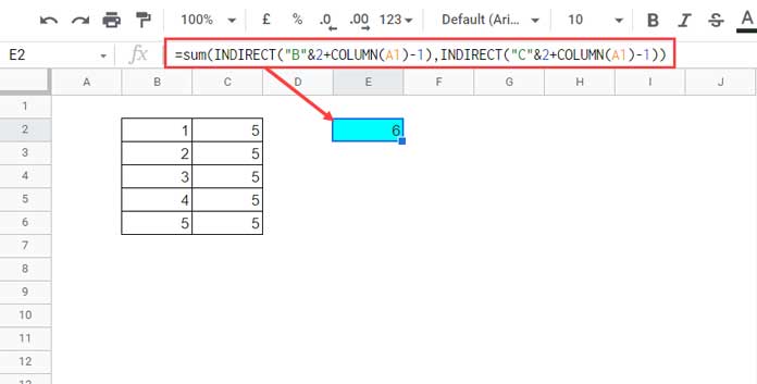
I want the row total column-wise. I mean 1+5 in E2, 2+5 in F2, 3+5 in G2, and so on.
In cell E2, insert the following Indirect and Column combo and copy-paste it across.
1. SUM, INDIRECT, and COLUMN:
=sum(INDIRECT("B"&2+COLUMN(A1)-1),INDIRECT("C"&2+COLUMN(A1)-1))Alternative Formulas:
2. SUM, INDEX, and COLUMN:
=sum(index($B$2:$C$6,column(A1)))3. SUM, OFFSET, and COLUMN:
=sum(offset($B$2:$C$4,column(A1)-1,0,1,2))The above formulas are as per our earlier three combinations, which we have used to get the reference down when we drag the formula across.
The only addition is the use of the function SUM.
You can drag the above formulas across and get the row reference from down.
Here also, we can use the TRANSPOSE.
=ArrayFormula(transpose(B2:B6+C2:C6))If you have several columns, I suggest using formulas 2 or 3 as they are easy to modify.
If you want an array formula as an alternative to TRANSPOSE, then use MMULT.
=ArrayFormula(transpose(mmult(B2:C6,sequence(columns(B2:C2))^0)))In this also, unlike TRANSPOSE, you can easily refer to several columns in a flash.
That’s all about dragging a formula across and getting the row reference from down.
Thanks for the stay. Enjoy!