


We can use the STDEVA function in Google Sheets to calculate the standard deviation of a sample (a small portion of a population)
It’s one of the useful Statistical functions in Google Sheets to measure the volatility of an investment.
A smaller standard deviation (SD/Std Dev) tells the investor that his investment is stable. If the standard deviation is 0, that means there is no volatility.
Is that the only purpose?
Nope! For example, we can use the STDEVA function to find out how the heights of a bunch of trees are spread out from their average (mean) height.
There are a couple of functions to estimate the standard deviation of a sample in Google Sheets.
Some are for backward compatibility or to solve the compatibility issue with similar applications.
Some others are for applying in a specific type of sample dataset. I mean when cells are hidden or when the sample is arranged as a database type table.
Also, the functions may treat texts and Boolean Values (Logical Values) TRUE or FALSE differently.
What are those different functions?
The functions are STDEVA, STDEV, STDEV.S, DSTDEV, SUBTOTAL.
The STDEVA function in Google Sheets stands out from the rest because it converts text values to 0 when others ignore them. The same is the case with Logical values.
STDEVA – Syntax and Arguments
Syntax:
STDEVA(value1, [value2, …])value1 – The first value or range/array of the sample.
value2, … – Additional values or ranges/arrays to include in the sample.
Examples to STDEVA function in Google Sheets
Here a few basic examples.
=STDEVA(5)The result of the above formula would be #DIV/0! Because the function requires at least two values to calculate the Std Dev.
=stdeva(5,10,15)SD = 15
In the above formula value1=5, value2=10, and value3=15.
Here is another example.
=stdeva(5,10,15,FALSE)SD = 6.454972244
The above formula is equal to using =stdeva(5,10,15,0)
What about the below STDEVA formula?
=stdeva(5,10,15,TRUE)SD = 6.075908711
The same is equal to using =stdeva(5,10,15,1)
As I have already mentioned above, the STDEVA function in Google Sheets will consider each text value as 0 for calculation. But that’s when you use a range/array reference.
The formula will return #VALUE! when you hardcode text inside the formula as =stdeva(5,10,"nil",1)
Volatile and Stable Stock
Here are two examples.
In the first array in A3:A6, the values indicate that they are relatively stable. In the second array in E3:E6, the values indicate big swings (volatility).
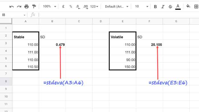
The formula in cell B3 returns 0.479 as the Std Dev. It’s close to 0, so stable.
In the second example (F3 formula), the Std Dev is 25.10. It’s farther from 0, so volatile.
Similar Functions and How They Differ From STDEVA in Google Sheets
You can learn more about the standard deviation by searching online.
So in the above part, I have concentrated mainly on how to use the STDEVA function in Google Sheets.
Also, we should avoid confusion using it as there are other similar functions. I hope the below examples will address it.
Please note, we are only talking about calculating the SD of a sample population.
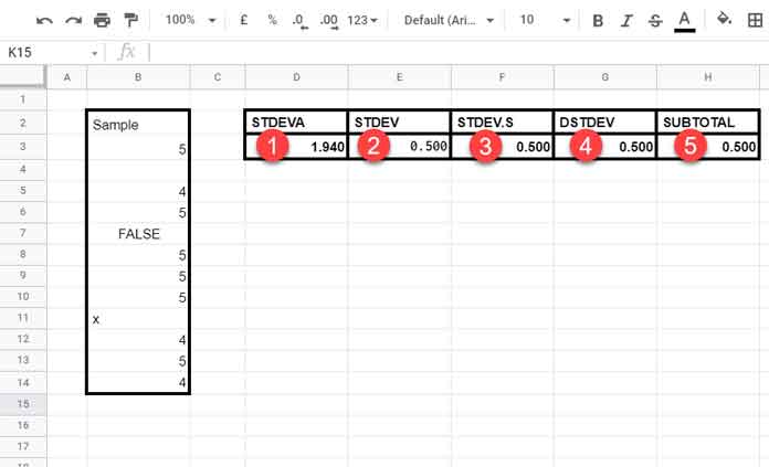
There are five formulas.
1. STDEVA formula in cell D3
=STDEVA(B3:B14)It excludes the blank cell B4 but treats B7 and B11 as zeros.
2. STDEV formula in Cell E3.
=STDEV(B3:B14)It excludes the blank cell B4, logical value in cell B7, and text value in cell B11.
If you want to replace it with the STDEVA function in Google Sheets, include FILTER with it (just for understanding the difference).
=stdeva(filter(B3:B14,isnumber(B3:B14)))3. STDEV.S formula in cell F3.
=STDEV.S(B3:B14)It’s the same point#2 function.
4. DSTDEV formula in cell G3.
=DSTDEV(B2:B14,1,{"Sample";if(,,)})It’s a database function that requires field labels. So included the label in B2 with the array. Unlike other functions, it takes conditions as an argument.
5. SUBTOTAL (Function No. 7 or 107)
=subtotal(107,B3:B14)To calculate the SD of visible cells.
That’s all. Thanks for the stay. Enjoy!
Related: Mean and Standard Deviation Straight Lines on a Column Chart in Google Sheets.