


In a vertical lookup, using the Vlookup function, the first column in the range will always be the search column. In certain cases, you may want to use the second, third or any nth column as the search column. Let’s see how to get dynamic search column in Vlookup in Google Sheets.
In my approach that using the nth column as the Vlookup search column, all the columns in the range must have unique column names (field labels).
You May Like: Column Heading | Column Label | Column Name | Field | Field Label in Google Sheets.
I am taking into account the following two scenarios in my examples to the dynamic search column in Vlookup.
- Search column controlled by the input value in a cell.
- Search and Index (output) columns controlled by input values in cells.
I am going to explain this under separate subtitles below.
Search Column Controlled by an Input Cell in Vlookup
Assume you want to return the price of an item based on either item name or item code.
In such a case, if the first column is for item name and the second column is for item code, how to dynamically control the search columns in Vlookup between these two columns.
Here is one example (GIF) to dynamic search column in Vlookup in Google Sheets.
Vlookup picks the search column based on the input value in cell E2 which is the column name. How? Please read on to know about that more.
Using the Filter function we can filter a single column or row. Here is an example to single column filter in Google Sheets.
Example to Single Column Filter in Google Sheets
Let’s use the above-provided sample dataset. The following formula filters column 2 in the range A2:D for the value 2.
=filter(A2:D,B2:B=2)The above filter formula will populate the below single row output.
| Gravel 10-20 mm | 2 | 2500 | 2.25 |
Example to Single Row Filter in Google Sheets
Unlike the single column filter, the filter criteria range will be a single row here. The below formula filters the first row (A2:D2) for the value “Item Code” which is column name.
=filter(A2:D,A2:D2="Item Code")The above filter formula will return a single column output.
| Item Code |
| 1 |
| 2 |
| 3 |
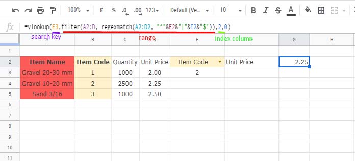
To get a dynamic search column in Google Sheets Vlookup, we can use the above second filter but with some minor modification.
In the second filter, the criterion is “Item Code”. Assume that criterion is in cell E2. Then the Filter would be as below.
=filter(A2:D,A2:D2=E2)So far so good, right?
We have now one column that changes based on the value in E2. join the Vlookup Index column to this output using Curly Braces. Then we will have a two-column array to use as Vlookup range.
I am joining the “Unit Price” column, which is going to be my Vlookup output column, here.
={filter(A2:D,A2:D2=E2),D2:D}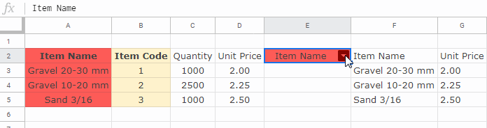
We have now a dynamic range to use in Vlookup. Here is that Vlookup formula with dynamic search column in Google Sheets.
=vlookup(E3,{filter(A2:D,A2:D2=E2),D2:D},2,0)Put your Vlookup criterion, i.e. search key, in cell E3 based on the column you choose in cell E2. That’s all.
Dynamic Search and Index Columns in Vlookup in Google Sheets
This is a more advanced version of the above Vlookup. Here in addition to the search column, the index column, i.e. output column, is also dynamic.
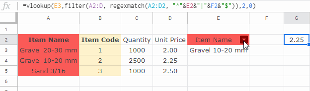
Here we must make some changes in the Filter formula as below. Instead of the above Filter, we can use this alternative formula that contains Regexmatch.
=filter(A2:D, regexmatch(A2:D2, "^"&E2&"|Unit Price$"))Related Reading: Regexmatch in Filter Criteria in Google Sheets [Examples].
This Filter and Regex combo has one advantage. It can dynamically control the search as well as the Index columns in Vlookup in Google Sheets.
Right now it’s not dynamic. It’s just a replacement to the filter we have used in the earlier Vlookup.
How to make this filter dynamic?
First, replace “Unit Price” (output column) in the regex with the cell reference F2. Then enter the key “Unit Price” in cell F2.
=filter(A2:D, regexmatch(A2:D2, "^"&E2&"|"&F2&"$"))Use this as the Vlookup Range. You have done!
How to use this Vlookup formula dynamically?
- To change the search column dynamically, change the value in E2. In E2 use either “Item Name” or “Item Code”.
- To change the Index/output column dynamically, change the value in F2. in F2 use either “Quantity” or “Unit Price”.
Follow this method to control the Vlookup search column and index column dynamically in Google Sheets.
Additional Resources: