


TRUE is a Boolean value which represents one of the truth value of logic. The other truth value aka logical value is FALSE. You can get the TRUE Boolean value by using the TRUE logical function in Google Sheets.
Instead of using the TRUE() function, you can simply put TRUE (without double or single quotes) in most of the cases in Google Sheets. Google Sheets will interpret such input values as Boolean values.
You can add, subtract, divide Boolean values as the TRUE has numeric value 1 and FALSE has 0.
Example Formula:
=TRUE()+TRUE()Result: 2
Here are a few examples of inputting or generating TRUE truth value in Google Sheets.
- Using an Expression, e.g., key the value 10 in cell A1 and use the formula
=A1=10or=eq(A1,10)in any other cell. This will return the value TRUE. - Enter the string TRUE or true in any cell. Google Sheets will treat this value as a Boolean TRUE value. To test this, enter TRUE in cell A1. In cell B1, use the formula
=A1+1. It will return 2 as TRUE is equal to 1. - Entering the
=TRUE()Logical Function in any cell will return the Boolean TRUE value.
Syntax:
true()Arguments:
There is no argument to use. So let’s go to some of the real-life use of the function TRUE in Google Sheets.
How to Use the TRUE Function in Google Sheets
The Boolean values are primarily associated with conditional statements. So you can use the TRUE function in conjunction with other logical functions like IF, NOT, AND, OR, IFERROR, IFNA, etc.
You May Like: Combined Use of IF, AND, OR Logical Functions in Google Sheets.
TRUE with IF in Docs Sheets
Assume cell A2 has a student name and cell B2 has his mark which is 60. In cell C2, use the below formula to test whether the mark is above 50.
=if(B2>50,true())This IF formula will return the Boolean TRUE value since the mark in cell B2 is >50.
If the value is <=50, then the formula would return the ‘other’ truth value which is FALSE. No need to specify FALSE() for this like =if(B2>50,true(),false()).
If you don’t want the false(), then put a comma after the true() as =if(B2>50,true(),).
Instead of using true() you can simply use the string true or TRUE without quotes around it.
Correct:
=if(B2>50,true)Incorrect:
=if(B2>50,"true")TRUE with AND, OR, IFERROR in Docs Sheets
The formula to return a TRUE Boolean value if all the marks in cell B2, C2, and D2 are above 50. Here I am using the AND operator with IF.
=if(and(B2>50,C2>50,D2>50),true())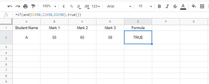
Similarly, you can use the TRUE function with the OR operator. Here is the formula to return TRUE Boolean if any of the marks in the said cells are above 50.
=if(OR(B2>50,C2>50,D2>50),true())Here is one more example, using the Iferror function.
=iferror(F3,true())This formula will return TRUE if cell F3 contains any error values.
From the above examples, one thing is obvious. In Google Sheets, you can use the string TRUE instead of the function TRUE(). Let me show you two instances where both behave differently.
Logical Function TRUE in Inserting Tick Boxes That Can’t Be Toggled
In cell C2, enter TRUE and in cell D2 enter either =TRUE or =true(). Select both of these cells. Then go to the menu Insert > Tick box.
This will insert two tick boxes. The first one you can toggle with a mouse click but the second one can’t be toggled.
Query Where Clause and Boolean Values
In my tutorial, i.e, on the use of literals in Query, you can see how to use TRUE boolean literal.
The correct way to use Boolean literal TRUE in Query Where clause is as below.
=QUERY(A2:B,"Select * where B=TRUE")Here you can’t use the formula as given below
=QUERY(A2:B,"Select * where B=TRUE()")That’s all about the role of TRUE logical function in Google Sheets.