HomeGoogle DocsSpreadsheetHow to Do a Reverse Hlookup in Google Sheets

How to Do a Reverse Hlookup in Google Sheets

Published on

Reverse Hlookup in Google Sheets is possible. To do this, you only need to rearrange the rows ‘virtually’. I mean there are no changes to the row position physically. Just change it within the Hlookup itself. How?

I’m trying to shed some light on this topic this time. See below how to do a reverse Hlookup in Google Sheets.

Reverse Hlookup in Google Sheets – What’s It?

Normally Hlookup searches across the first row for a key. In reverse Hlookup, instead of the first row, we can use any other row. But remember, there is no reverse Hlookup function!

How is Reverse Hlookup Possible in Google Sheets?

As an example, we can use Hlookup to search across the third row and return the value from the first row by rearranging the data within Hlookup. It’s very simple.

Google Sheets Reverse Hlookup Formula Example

See the below sample data.

Google Sheets Reverse Hlookup Formula Example

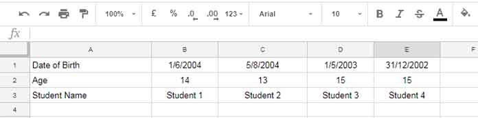
In this, I want to find the ‘date of birth’ of “Student 2”. That means “Student 2” is the search key in Hlookup. But it’s in the third row.

Hlookup can only search across the first row. In order to do a reverse Hlookup in Google Sheets first rearrange the data as below (this we want to do within Hlookup).

{A3:E3;A1:E2}

You should apply this formula within the Hlookup as the range. By doing so, Google Sheets places the third row above the first row. Now the column with the names is in the first row and the row containing the ‘date of birth’ is the second row.

In this new range, Hloookup is possible. See the reverse Hlookup formula now.

=HLOOKUP("Student 2",{A3:E3;A1:E2},2,false)

This formula, as usual searches across the first row for the student name “Student 2” and returns the date of birth from the second row. It is possible with the rearranging of rows.

In concise, whenever you want to do a reverse/backward Hlookup, rearrange the rows in your data that within the Hlookup formula.

Similar:

  1. Vlookup in Google Sheets – 10 Formula Variations, Tips, and Tricks.
  2. How to Return an Entire Column in Hlookup in Google Sheets.
Prashanth KV
Prashanth KV
Your Trusted Google Sheets and Excel Guide Prashanth KV brings a wealth of experience in Google Sheets and Excel, cultivated through years of work with multinational corporations in Mumbai and Dubai. As a recognized Google Product Expert in Docs Editors, Prashanth shares his expertise through insightful blogging since 2012. Explore his blog for practical tips and guidance on maximizing your spreadsheet skills.

Dynamic Sum Column in SUMIF in Google Sheets

To obtain a dynamic sum column (sum_range argument) in SUMIF, we can utilize the...

Create a Calendar in Excel with a One-Line Dynamic Array Formula

This tutorial explains how to create a calendar in Excel using a one-line formula...

Excel: Month Name to Number & Number to Name

This tutorial showcases the most efficient formulas for converting a month name to a...

Get the First or Last Row/Column in a New Google Sheets Table

If you've recently started using the new Google Sheets TABLE functionality, you may find...

More like this

Dynamic Sum Column in SUMIF in Google Sheets

To obtain a dynamic sum column (sum_range argument) in SUMIF, we can utilize the...

Get the First or Last Row/Column in a New Google Sheets Table

If you've recently started using the new Google Sheets TABLE functionality, you may find...

UNIQUE Function in Visible Rows in Google Sheets

The UNIQUE function doesn't inherently include only visible rows when it returns values, discarding...

LEAVE A REPLY

Please enter your comment!
Please enter your name here

This site uses Akismet to reduce spam. Learn how your comment data is processed.