It’s not easy to provide a tailor-made formula for comparing tables and removing duplicates in Google Sheets.
It’s mainly because the requirements may vary from person to person.
Here I will share a formula to help you compare two tables and remove duplicates in Google Sheets.
This tutorial can help you in the following way.
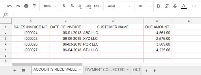
Suppose you have two tables in a Google Sheets file containing the invoice raised, and payment received details.
Assume the corresponding tab names are ACCOUNT RECEIVABLE and PAYMENT COLLECTED.
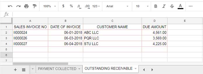
How to match the invoice numbers and remove the matching ones?
You can compare two tables for duplicates and remove them using a formula in Google Sheets.
Let’s prepare the sample data first.
Sample Data for Comparing Two Tables and Removing Duplicates
Table 1: ACCOUNTS RECEIVABLE
I have the following records in the accounts receivable tab.

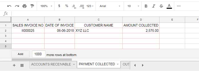
Table 2: PAYMENT COLLECTED
I have just one record in the payment collected tab.

You can see now how to compare these two tables for duplicates and remove them.
As you can see Invoice Number II000025 repeats in both tables.
We can handle it in two ways!
- Remove all the occurrences of the matching rows.
- Keep one record of the matching row.
How do we match the records?
It’s up to you whether to consider only the invoice number for matching (method A) or the total row (method B).
Formulas for Comparing Two Tables and Removing Duplicates
1. Removing All Occurrences of the Matching Row
Matching Total Row (method B):
The following formula will remove matching rows from both tables.
=unique(vstack('ACCOUNTS RECEIVABLE'!A2:D,'PAYMENT COLLECTED'!A2:D),,true)The VSTACK appends both tables vertically. The UNIQUE returns the distinct rows.

Here we can also use the following QUERY formula.
=query(query(vstack('ACCOUNTS RECEIVABLE'!A1:D,'PAYMENT COLLECTED'!A2:D),"Select Col1,Col2,Col3,Col4, Count(Col1) where Col1<>'' group by Col1,Col2,Col3,Col4"),"Select Col1,Col2,Col3,Col4 where Col5=1")How Does this Query Formula Compare Two Tables (Datasets) and Remove Duplicates?
Before using this formula, it’s good for you to understand its logic first.
The above is a nested Query formula. The inner Query formula is the main one. What does it do?
=query(vstack('ACCOUNTS RECEIVABLE'!A1:D,'PAYMENT COLLECTED'!A2:D),"Select Col1,Col2,Col3,Col4, Count(Col1) where Col1<>'' group by Col1,Col2,Col3,Col4")It groups all columns in the table and returns the count of records as follows.

The Outer Query filters out any row that contains >1 in the last column.
Matching Invoice Number (method A):
Assume the invoice amount is different for II000025 in both tables.
The above formulas won’t remove the said invoices because they are distinct.
In this case, we can modify our earlier Query formula by grouping only the invoice column.
=query(query(vstack('ACCOUNTS RECEIVABLE'!A1:D,'PAYMENT COLLECTED'!A2:D),"Select Col1,max(Col2),max(Col3),max(Col4), Count(Col1) where Col1<>'' group by Col1"),"Select Col1,Col2,Col3,Col4 where Col5=1")2. Keeping the First Occurrence
Here also, we can use two types of formulas: Consider only the invoice number for matching (method A) or the total row (method B).
Matching Total Row (method B):
=let(ftr,unique(vstack('ACCOUNTS RECEIVABLE'!A2:D,'PAYMENT COLLECTED'!A2:D)),filter(ftr,choosecols(ftr,1)<>""))Here the Unique does the job. The purpose of LET is to filter out blank rows in the result.
Matching Invoice Number (method A):
=let(ftr,sortn(vstack('ACCOUNTS RECEIVABLE'!A2:D,'PAYMENT COLLECTED'!A2:D),9^9,2,1,1),filter(ftr,choosecols(ftr,1)<>""))Here the SORTN takes the place of Unique.
Related: SORTN Tie Modes.
The highlighted number in the formula represents the column for matching. Here it’s the invoice column, so # 1.
That’s all about how to compare two tables and remove duplicates in Google Sheets.


