


The use of AND Logical function in an array is a little tricky. Unlike OR logical, you can’t use it with a nested IF to get expanded results. Then how to use AND Logical in Array in Google Sheets.
You can’t use AND to get an expanded result. But there is an alternative way to get the same result in Google Sheets. This is very important to learn as it can come very useful for you. Here is that use.
AND Logical Function in Expanding Array in Google Sheets
For example, I want to return TRUE if the values in cell A2, as well as in cell B2, is greater than 0. First a normal AND logical test.
=if(and(A2>=0,B2>=0),TRUE,FALSE)The above logical test would return TRUE or FALSE based on the values in the said cells. But I want the result to be expanded to rows below. Because I want to test the values in A3 and B3, A4 and B4 and so on.
That means I want to use AND logical in Array in Google Sheets. Here is an example formula.
This ArrayFormula is an example of how to use AND logical in Array in Google Sheets. Seems little complicated, right? Don’t worry. I’ll explain it.
AND Array Formula Explanation
Assume the value in cell A2 is 5 and cell B2 is 6. So the below formula in any cell would return 1.
Formula:
=(A2>0)*(B2>0)Result:
TRUE x TRUE = 1
But when you want to use it in an array the formula would be as below.
=ArrayFormula(if(len(A2:A),(A2:A>0)*(B2:B>0),""))Now you may want to know why I’ve used IF and LEN functions, I mean the if(len(A2:A), in this formula.
Actually, you can replace the IF+LEN combo using if(A2:A<>"", as both are meant for the same thing. What is that?
The use of the above combo in the formula is to limit the expansion of the formula results based on the range. Because we have used an infinite range in the formula like A2:A instead of using a fixed range like A2:A10 or something similar.
If you want more clarification on this you can refer my LEN function tutorial.
This’s the only possible way you can use AND logical in Array in Google Sheets. But the above formula would only return 1 for TRUE and 0 for FALSE. That’s enough for logical tests.
But if you are very much particular to get Boolean TRUE or FALSE, you can use the following AND Array Formula.
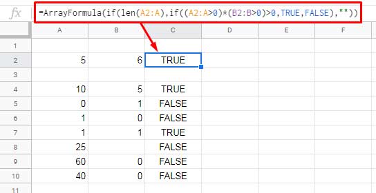
=ArrayFormula(if(len(A2:A),if((A2:A>0)*(B2:B>0)>0,TRUE,FALSE),""))OR
=ArrayFormula(if(A2:A<>"",if((A2:A>0)*(B2:B>0)>0,TRUE,FALSE),""))Hope you’ve enjoyed the above tips. See you again with another awesome Google Spreadsheet Tutorial.
So I have ArrayFormula checking Column C Price to see what range it falls in. Then it assigns the number based on that range it puts it in Column M. It works perfectly as a formula, but when I make it an array, it just posts all Zeros. So not seeing any in the range, but they all are. I love your site and have search it but couldn’t figure it out. Thank you.
Note:- Formula removed by admin due to improper formatting.
Hi, Tim Murray,
Sorry that my editor sometimes automatically removes the greater than or equal to operators. Anyhow, I have got your mail with the correct formula. I will check it later and reply back.
Hi, Tim Murray,
This may help.
={"Price Range ID";ArrayFormula(if(C2:C>0,IF(C2:C<150001,1,IF(C2:C<250001, 2, IF(C2:C<350001,3, IF(C2:C<450001,4, IF(C2:C<=550001,5, IF(C2:C<=650001,6, IF(C2:C<750001,7, IF(C2:C<900001,8, IF( C2:C<1200001,9,0))))))))),))}The AND operator in your formula won't support the array formula.
Actually, the said logical operator is not required in your formula.
Hi,
Your info is a true inspiration. can you help me, please? My formula is;
=IFS(N2:N=20000000;N2:N=100000000;N2:N=300000000;N2:N=500000000;N2:N=700000000;N2:N=1000000000;
3250000+(0,5%*N2:N))
How to use it in the array formula? Thanks.
Hi, Rahmat Jaenudin,
See if this formula helps?
=ArrayFormula(IF((N2:N=20000000)+(N2:N=100000000)+(N2:N=300000000)+(N2:N=500000000)+(N2:N=700000000)+(N2:N=1000000000)>=1;3250000+(0,5%*N2:N);))I’ve shortened it to this:
=Arrayformula(if(B4:B76*B3:B75>0,B4:B76-B3:B75,""))I’ve needed it to subtract earlier time from later time to get the duration of an activity performed during that time. Basically B4-B3, B5-B4 etc. – but only if both of the cells in subtraction are not empty, in order to keep result column clean. It worked.
Thanks for the guidance and inspiration and – what do you think? 🙂
Hi, Dodo Phe,
I think your formula may not work as desired.
Check the output properly. You may need a more complicated formula.
=Query(ArrayFormula(IFERROR(IF(ISEVEN(if(len(B4:B),row(B4:B),))=true,B4:B,)-IF(ISODD(if(len(B3:B),row(B3:B),))=true,B3:B,))),"Select * where Col1>0")Best,
Prashanth KV