How to Use the XNPV Function in Google Sheets

The XNPV function in Google Sheets, one of its financial functions, is used to calculate the net present value for a schedule of irregularly spaced cash flows.

If the cash flows are periodic (i.e., evenly spaced), you can use the regular NPV function instead. You’ll find a brief NPV vs XNPV comparison toward the end of this tutorial.

To calculate XNPV, we must provide three inputs:

a discount rate,
a range of cash flow amounts, and
a matching range of dates.

Table of Contents

What Is Net Present Value (NPV) in Simple Terms?

Net Present Value, or NPV, is a way to measure how much future money is worth today.

Imagine you’re set to receive $5,000 from a project one year from now. It sounds valuable—but if you had that $5,000 today, you could invest it and earn interest.

So, the future $5,000 isn’t worth the same as $5,000 today. Net present value (NPV) helps calculate how much that future amount is really worth right now.

Why Use XNPV Instead of NPV?

Most financial calculators—and even the NPV function in Google Sheets—assume that cash flows occur at regular intervals. But in real life, payments or receipts often happen on irregular dates.

That’s where the XNPV function in Google Sheets is more useful. It accounts for the exact dates of each cash flow, making the net present value calculation more accurate.

XNPV Function in Google Sheets – Syntax and Arguments

Syntax:

XNPV(discount_rate, cashflow_amounts, cashflow_dates)

Arguments:

discount_rate – The rate used to discount the future cash flows.
cashflow_amounts – The series of incoming or outgoing cash flows, where positive values represent income (cash inflows) and negative values represent payments or costs (cash outflows).
cashflow_dates – The dates corresponding to the cash flows.

Additional Details

In the XNPV function, the dates must include a starting point, and all subsequent dates should be on or after this first date. However, they don’t need to be in chronological order.
If the first cashflow_amount represents an initial investment or cost, enter it as a negative value.
All cash flows are discounted using a 365-day year.

XNPV Formula Example in Google Sheets

In the example below:

The discount rate (10%) is in cell A5.
Cash flow values are in B5:B10.
Corresponding dates are in C5:C10.

The value in B5 is negative, representing the initial investment.

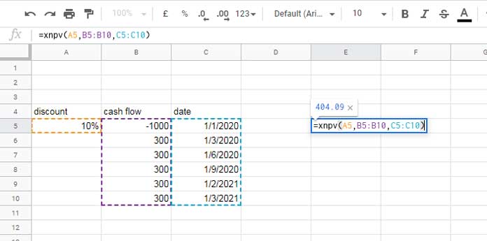
XNPV function example in Google Sheets showing cash flows, dates, and calculated result

Formula:

=XNPV(A5, B5:B10, C5:C10)

If the dates in C5:C10 were at regular intervals (e.g., 01/01/2020, 01/01/2021, …, 01/01/2025), then the NPV function would be appropriate instead of XNPV.

Here’s how you would use NPV in that case:

=NPV(A5, B6:B10) + B5

The NPV and XNPV functions would both return 137 in this scenario.

NPV vs XNPV in Google Sheets

Use NPV when:

The cash flows occur at regular intervals (monthly, yearly, etc.).

Use XNPV when:

The cash flows occur at irregular intervals, such as varying payment or income schedules.

Conclusion

If the result of your XNPV formula in Google Sheets is negative, the project may not be financially viable—it indicates a net cash outflow over time.

But if the net present value is positive, as in our example, the project may be worth pursuing. The larger the positive result, the greater the potential benefit to the business.

You can even combine XNPV with IF to make decision-making easier at a glance. For example:

=IF(XNPV(A5, B5:B10, C5:C10) > 0, "Can consider")

Or try using a star rating system to visually assess profitability:

=LET(val, XNPV(A5, B5:B10, C5:C10),
 IF(val > 1000, "★★★★★",
 IF(val > 500, "★★★★",
 IF(val > 100, "★★★",
 IF(val > 0, "★★", "Quit")))))

That’s it on the XNPV function in Google Sheets. If your cash flows aren’t on a neat schedule, this one’s for you.