You can use XMATCH in visible rows—i.e., XMATCH in filtered data in Google Sheets—without relying on a helper column. The formula automatically excludes hidden rows from its match range.

This method is specifically for matching search keys in a column and returning their relative positions—or returning #N/A if no match is found.

While the relative position might not matter in many use cases, some scenarios require it. If you do care about that position, it’s important to understand how it changes when rows are hidden.

I’ll explain that first, and then show you how to XMATCH visible rows in Google Sheets.

Hidden Rows and Relative Position

Below is a list of dates in the range B2:B11. In A2:A11, I’ve noted their relative positions.

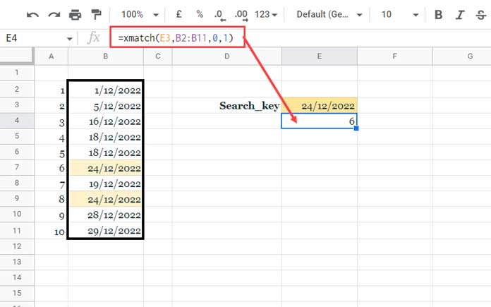
Example:

The relative position of 24/12/2022 in B2:B11 is 6 when searched from top to bottom.

Formula #1 (in E4):

=XMATCH(E3, B2:B11, 0, 1)

If you hide row 7, the result remains 6, because XMATCH doesn’t ignore hidden rows by default.

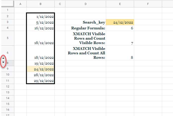
But what if you want the position of the next visible match?

That’s what we mean by XMATCH visible rows in Google Sheets.

Let’s say row 7 (which contains 24/12/2022) is hidden. The formula should now match the next visible 24/12/2022, say in row 9. The full row count position is 8, but among visible rows only, it’s 7.

How to XMATCH in Filtered Data in Google Sheets

We’ll explore two methods depending on whether you want to count:

1. All rows (visible + hidden)
2. Only visible rows

1. XMATCH Visible Rows, Counting All Rows

This is similar to using XLOOKUP in filtered data. To make XMATCH work with filtered or hidden rows, we’ll use:

• BYROW (a LAMBDA helper function)
• SUBTOTAL (to identify visible rows)

Helper Formula:

BYROW(B2:B11, LAMBDA(range, SUBTOTAL(103, range)))

This returns 1 for visible cells and 0 for hidden ones.

We can use this result to build a virtual lookup range by replacing hidden rows with blank values:

IF(helper_formula_result = 0, "", B2:B11)

Formula #2 (in E6):

=ARRAYFORMULA(XMATCH(E3, IF(BYROW(B2:B11, LAMBDA(range, SUBTOTAL(103, range)))=0, "", B2:B11), 0, 1))

Here’s the breakdown:

• search_key: E3
• lookup_range: modified using IF and BYROW
• match_mode: exact match (0)
• search_mode: top to bottom (1)

We use ARRAYFORMULA to ensure the IF expression returns an array that XMATCH can process correctly.

2. XMATCH Visible Rows, Counting Only Visible Rows

In this version, we’ll exclude hidden rows from the result count by using FILTER instead of IF.

Formula #3 (in E5):

=XMATCH(E3, FILTER(B2:B11, BYROW(B2:B11, LAMBDA(range, SUBTOTAL(103, range))) > 0), 0, 1)

No need for ARRAYFORMULA, as FILTER handles arrays naturally.

Note: Make sure the range B2:B11 does not contain empty cells. If it does, the formula may return an incorrect position or fail to match the value.

Reverse Search: From Bottom to Top

Sometimes, your data is sorted with the latest entries at the bottom, and you want to search upward.

To do that, just change the search_mode argument from 1 to -1.

=XMATCH(E3, B2:B11, 0, -1)
=ARRAYFORMULA(XMATCH(E3, IF(BYROW(B2:B11, LAMBDA(range, SUBTOTAL(103, range)))=0, "", B2:B11), 0, -1))
=XMATCH(E3, FILTER(B2:B11, BYROW(B2:B11, LAMBDA(range, SUBTOTAL(103, range))) > 0), 0, -1)

Test these formulas in your own Sheet for better clarity.

Conclusion

Using XMATCH in filtered data in Google Sheets unlocks a lot of flexibility. Whether you want to match visible entries and count all rows—or just the visible ones—you now have working formulas for both.

This guide shows how to control XMATCH behavior without any helper columns, by using dynamic formulas.

Thanks for reading!

Related Resources

• XMATCH First or Last Non-Blank Cell in Google Sheets
• XMATCH Multiple Columns in Google Sheets
• XMATCH vs MATCH in Excel (New vs Old)
• XMATCH Row by Row: Finding Values Across a Range in Google Sheets
• How to Use OFFSET and XMATCH Functions Together in Excel
• Sort by Field Labels Using the SORT and XMATCH Combo in Excel