Do you know how to use the XMATCH function to find the first or last non-blank cell in Google Sheets? Also, how to highlight those cells?

You might still be using old-school approaches like logical tests combined with MATCH for this task.

For example, you can see such an approach here: Find the Last Non-Empty Column in a Row in Google Sheets. Of course, that still works well.

But if you want to learn newer, more efficient ways to do things in spreadsheets, you’ll like this XMATCH approach.

We’ll leverage the wildcard matching and reverse lookup features of XMATCH.

Using XMATCH to find the first or last non-blank cell in a row or column has several advantages.

First and foremost, it helps identify the start and end rows or columns of your data range.

Beyond that, it’s useful for highlighting those specific cells and for limiting the spill range of formulas like ARRAYFORMULA and LAMBDA.

For example, if you have values in column A, instead of using the open-ended range A1:A, you can specify a dynamic range like this:

=ARRAYFORMULA(INDIRECT("A1:A"&last_non_blank_cell))

This way, your array formula will stop spilling at the last non-blank cell, preventing #REF! errors in cells beyond the data range.

XMATCH Last Non-Blank Cell in a Column in Google Sheets

Usually, you might scroll horizontally or vertically to locate the last non-empty cell in a row or column.

This can be time-consuming, especially when dealing with large datasets spanning hundreds of rows or columns.

Also, scrolling won’t help if you want to highlight the first or last non-blank cell automatically.

Let me use a small dataset to illustrate this with a screenshot and explanation.

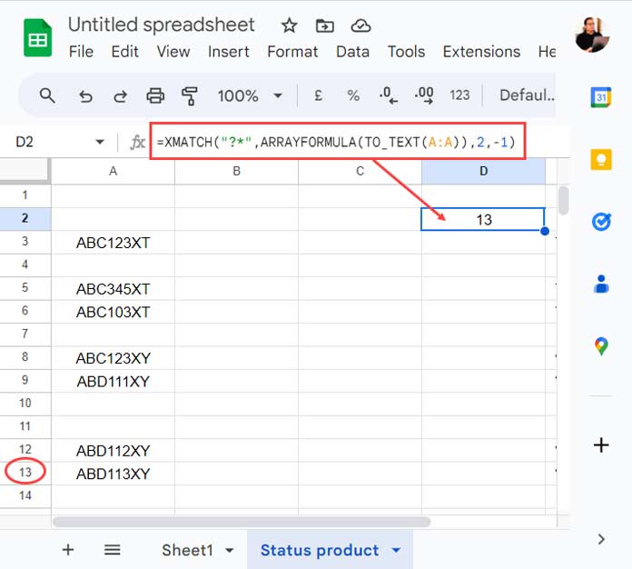
I have product codes in column A, with some blank cells in between. Regardless, I want to find the last code.

Assume the last non-blank cell in column A contains the code "ABD113XY", but we don’t know this value upfront.

If we did know the value, the formula would be simple:

=XMATCH("ABD113XY", A:A, 0)

But how do you use XMATCH to find the last non-blank cell in column A without knowing its value?

Here’s the answer:

=XMATCH("?*", ARRAYFORMULA(TO_TEXT(A:A)), 2, -1)

This formula returns the row number of the last non-empty cell in column A.

Formula Explanation: Wildcard Match and Null Values

Syntax: XMATCH(search_key, lookup_range, [match_mode], [search_mode])

• lookup_range: Here, I wrapped A:A in ARRAYFORMULA(TO_TEXT()) to convert all cells to text. This is essential to perform wildcard matching.
• This conversion turns blank cells into null values (empty strings).

Note: A null value is a zero-length string, so ISBLANK() returns FALSE, but LEN() returns 0.

• The asterisk * wildcard matches any number of characters, including zero, which means it would match blank cells as well.
• The question mark ? wildcard matches exactly one character.
• Combining ?* ensures the match only targets cells with at least one character, effectively ignoring blanks.
• The match_mode argument is 2, indicating wildcard matching.
• The search_mode argument is -1, which makes the search go from the last cell to the first (reverse search).

XMATCH Last Non-Blank Cell in a Row

To find the last non-blank cell in a row, use the same formula but adjust the range accordingly.

For example, this formula returns the relative position (column number) of the last non-empty string in the first row:

=XMATCH("?*", ARRAYFORMULA(TO_TEXT(1:1)), 2, -1)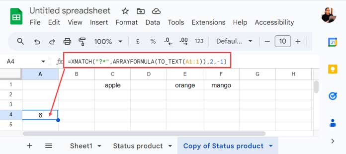

For the second row, change the range to 2:2.

Frequently Asked Questions

Q: Should the lookup array be sorted?
A: No, sorting isn’t necessary for this to work.

Q: Can I start the search from the nth cell instead of the first?
A: Yes. For example, A10:A will return the relative position within that range. Keep in mind it’s relative to the start of your range.

Q: Does this work with numbers, dates, times, and mixed data types?
A: Yes! The formula works regardless of the data type.

Q: What if the last non-empty cell contains an error?
A: By default, XMATCH treats error cells as blank. To consider error cells as non-blank, wrap your range with IFERROR, like this:

=XMATCH("?*", ARRAYFORMULA(TO_TEXT(IFERROR(A1:A, "."))), 2, -1)

XMATCH First Non-Blank Cell in Google Sheets

If you’ve followed everything above, you’ll find it easy to get the XMATCH first non-blank cell in Google Sheets too.

The only change is the last argument, the search mode.

Similar to XLOOKUP, XMATCH has four search modes:

• 1 (search from first to last),
• -1 (search from last to first),
• 2 (binary search ascending),
• -2 (binary search descending).

We used -1 for the last non-empty cell. Simply replace it with 1 to find the first non-empty cell.

First Non-Blank Cell in a Column:

=XMATCH("?*", ARRAYFORMULA(TO_TEXT(A:A)), 2, 1)

First Non-Blank Cell in a Row:

=XMATCH("?*", ARRAYFORMULA(TO_TEXT(1:1)), 2, 1)

Conditional Formatting: Highlighting First or Last Non-Blank Cells

You can use these XMATCH formulas to find the position of the first or last non-empty cell and highlight them with conditional formatting.

For highlighting the first or last non-blank cell in a row, use the COLUMN() function.

1. Go to Format > Conditional formatting.
2. Set “Apply to range” as A1:Z1.
3. Use these custom formulas:

Highlight First Non-Empty Cell in a Row:

=COLUMN()=XMATCH("?*", ARRAYFORMULA(TO_TEXT(1:1)), 2, 1)

Highlight Last Non-Empty Cell in a Row:

=COLUMN()=XMATCH("?*", ARRAYFORMULA(TO_TEXT(1:1)), 2, -1)

For highlighting in a column, replace COLUMN() with ROW(). For example, apply to range A1:A1000.

Highlight First Non-Empty Cell in a Column:

=ROW()=XMATCH("?*", ARRAYFORMULA(TO_TEXT(A:A)), 2, 1)

Highlight Last Non-Empty Cell in a Column:

=ROW()=XMATCH("?*", ARRAYFORMULA(TO_TEXT(A:A)), 2, -1)

Additional Resources

• XMATCH Visible Rows in Google Sheets
• XMATCH Multiple Columns in Google Sheets
• XMATCH vs MATCH in Excel (New vs Old)
• XMATCH Row by Row: Finding Values Across a Range in Google Sheets
• How to Use OFFSET and XMATCH Functions Together in Excel
• Sort by Field Labels Using the SORT and XMATCH Combo in Excel
• Find the Address of the Last Used Cell in Google Sheets
• Find the Last Used Row Number in Excel
• Find the Last Used Row’s Last Value Address in Excel