


We must follow a workaround solution to calculate the weighted average of filtered or visible data in Google Sheets. Why so?
SUMPRODUCT and AVERAGE.WEIGHTED, the popular two options, don’t support excluding hidden rows in the weighted average calculation.
The workaround involves identifying visible rows with the help of a SUBTOTAL and MAP array formula combination.
We will use that as a virtual helper column within the said two options.
Note:- You can check these functions in my Google Sheets function guide.
Before filtering or hiding rows, let’s understand the regular weighted average calculation.
Weighted Average = Sum (Data_Point_Value * Weight) / Sum(Weight)
Assume we have procured different quantities of a product at different unit prices.
Let’s see how to calculate the weighted average cost of the product per unit.
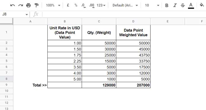
As per the above formula, the output will be;
Weighted Average = Sum (Data_Point_Value * Weight) / Sum(Weight) which is equal to 207000/129000 = 1.60 USD.
In Google Sheets, we can use the following formulas for this calculation.
Formula # 1 [AVERAGE.WEIGHTED]:
Syntax: AVERAGE.WEIGHTED(values, weights)
=AVERAGE.WEIGHTED(B2:B8,C2:C8)Formula # 2 [SUMPRODUCT]:
Syntax: SUMPRODUCT(values,weights)/sum(weights)
=SUMPRODUCT(B2:B8,C2:C8)/sum(C2:C8)How do we calculate the weighted average of filtered (visible) data then?
Calculating the Weighted Average of Filtered Data
We have the above table and want to exclude the last three purchases while calculating the weighted average cost of the product per unit.
We don’t want to delete rows 6, 7, and 8, instead, hide them using one of the available options: grouping, filtering, manual hide, or slicer.
The problem is that the above two Google Sheets formulas will return the same output as they can’t differentiate visible and hidden rows.
But there is a way to omit hidden rows while calculating the weighted average in Google Sheets.
The first step to calculating the weighted average of filtered data is to identify the visible rows in the range.
Note:- Here filtered means visible rows. You can use any available methods to hide rows and make only the required data visible.
The following MAP and SUBTOTAL combo will do that magic by returning 1 in visible rows and 0 in hidden rows.
=map(C2:C8,lambda(r,subtotal(103,r)))How do we include this technique in the earlier two formulas?
Here is the AVERAGE.WEIGHED formula approach to calculate the weighted average of the filtered data.
Syntax: index(AVERAGE.WEIGHTED(values, weights*map_subtotal_combo))
=index(AVERAGE.WEIGHTED(B2:B8,C2:C8*map(C2:C8,lambda(r,subtotal(103,r)))))Scroll up and take a look at formula # 1 and the just above formula, especially the highlighted part.
You can see that we have multiplied the weight with the hidden row identifier (combo formula) to return 0 (zero) in hidden rows.
We can also use this technique in SUMPRODUCT for calculating the weighted average of visible or filtered data in Google Sheets.
Syntax: SUMPRODUCT(values,weights,map_subtotal_combo)/SUMPRODUCT(weights*map_subtotal_combo)
=sumproduct(B2:B8,C2:C8,map(C2:C8,lambda(r,subtotal(103,r))))/sumproduct(C2:C8*map(C2:C8,lambda(r,subtotal(103,r))))That’s all. Thanks for the stay. Enjoy!
I am collating data across manufacturing units across multiple lines of a factory every day for 8 hours.
I can get a weighted avg for filtered rows. However, simultaneously, I need to calculate the weighted avg across all units for a particular day.
Hi, Raghavendra,
Please give me access to your sample data and expected results.
Then I will try.
Hi, can I have the above formula with the IF condition?
Please elaborate.
Thank you very much. I thought of using an excel array formula. However, it didn’t work! Thanks a ton, once again.